Inflow Performance Relation — SepalSolver

Definition: The Inflow Performance Relationship (IPR) describes the relationship between the bottom-hole flowing pressure ( $p_{wf}$ ) and the production rate ('math:q) of a well. It is a fundamental tool in reservoir engineering used to evaluate well productivity and forecast performance under different operating conditions.

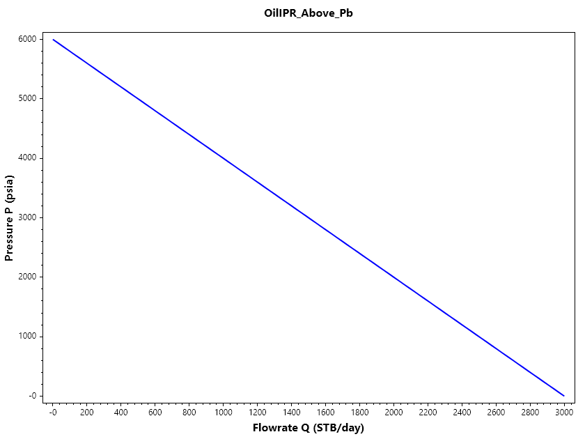
Oil Well IPR Above Bubble Point

the reservoir pressure is above the bubble point pressure, the fluid remains single-phase (oil only). The relationship is linear and can be expressed as:

q = J \cdot (p_r - p_{wf})

Where:

$q$ = production rate (STB/day)

$J$ = productivity index (STB/day/psi)

$p_r$ = average reservoir pressure (psi)

$p_{wf}$ = bottom-hole flowing pressure (psi)

Numerical Example:

Given:

$J = 2 \, \text{STB/day/psi}$

$p_r = 3000 \, \text{psi}$

$p_{wf} = 2500 \, \text{psi}$

q = 2 \cdot (3000 - 2500) = 1000 \, \text{STB/day}

Example 1C#

double J = 2; // STB/day/psi    
double p_r = 3000; // psi
double p_wf = 2500; // psi
double q = J * (p_r - p_wf); // STB/day
Console.WriteLine($"Production Rate (q) = {q} STB/day");
// Full Range
double qfun(double pwf) => J * (p_r - pwf);
ColVec Prange = Linspace(0, p_r);
ColVec Qrange = Arrayfun(qfun, Prange);
Plot(Prange, Qrange, "b", 2);
Xlabel("Flowrate Q (STB/day)");
Ylabel("Pressure P (psia)");
Title("OilIPR_Above_Pb");
SaveAs("OilIPR_Above_Pb.png");

OutputFrom the book

Production Rate (q) = 1000 STB/day

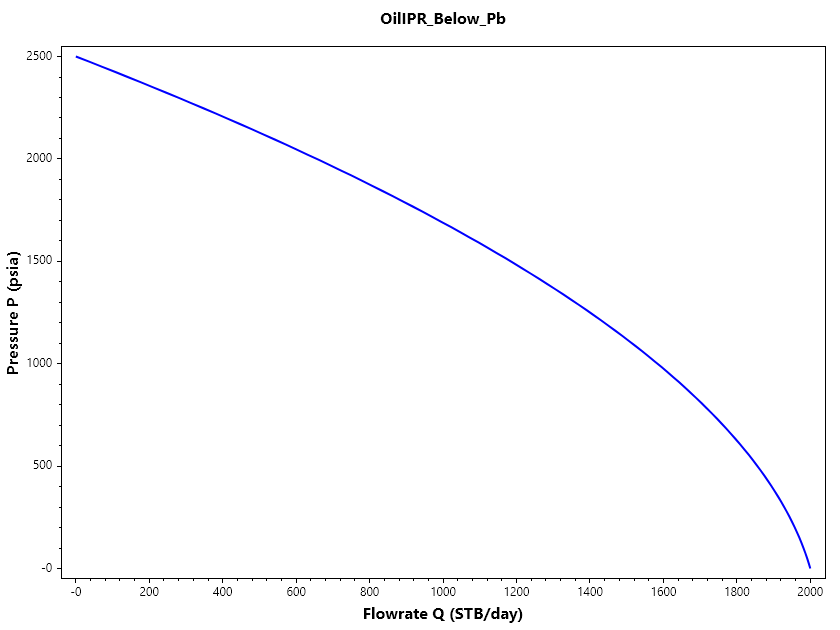
Oil Well IPR Below Bubble Point

When the reservoir pressure falls below the bubble point, gas evolves from solution, and the relationship becomes non-linear. Vogel’s empirical equation is commonly used:

\frac{q}{q_{max}} = 1 - 0.2 \cdot \frac{p_{wf}}{p_r} - 0.8 \cdot \left(\frac{p_{wf}}{p_r}\right)^2

Where:

- $q_{max}$ = maximum flow rate at $p_{wf} = 0$

Numerical Example:

Given:

$q_{max} = 2000 \, \text{STB/day}$

$p_r = 2500 \, \text{psi}$

$p_{wf} = 1000 \, \text{psi}$

\frac{q}{2000} = 1 - 0.2 \cdot \frac{1000}{2500} - 0.8 \cdot \left(\frac{1000}{2500}\right)^2\\ \frac{q}{2000} = 1 - 0.08 - 0.128 = 0.792\\ q = 2000 \cdot 0.792 = 1584 \, \text{STB/day}

Example 2C#

double q_max = 2000; // STB/day
double p_r = 2500; // psi
double p_wf = 1000; // psi
double q = q_max * (1 - 0.2 * (p_wf / p_r) - 0.8 * Pow(p_wf / p_r, 2)); // STB/day
Console.WriteLine($"Production Rate (q) = {q} STB/day");
// Full Range
double qfun(double pwf) => q_max * (1 - 0.2 * (pwf / p_r) - 0.8 * Pow(pwf / p_r, 2));
ColVec Prange = Linspace(0, p_r);
ColVec Qrange = Arrayfun(qfun, Prange);
Plot(Qrange, Prange, "b", 2);
Xlabel("Flowrate Q (STB/day)");
Ylabel("Pressure P (psia)");
Title("OilIPR_Below_Pb");
SaveAs("OilIPR_Below_Pb.png");

OutputFrom the book

Production Rate (q) = 1583.9999999999998 STB/day

Flow Efficiency and Skin

Flow Efficiency (FE): Flow efficiency is a measure of how effectively a well produces compared to an ideal, undamaged well. It is defined as:

FE = \frac{q_{actual}}{q_{ideal}}

Example 3C#

double q_ideal = 1584; // STB/day (from previous example)
double q_act = 1200; // STB/day (maximum flow rate)
double FE = q_act / q_ideal; // Flow Efficiency
Console.WriteLine($"Flow Efficiency (FE) = {FE:P2}");

OutputFrom the book

Flow Efficiency (FE) = 75.76%

Skin Factor (s): Skin represents additional pressure drop caused by near-wellbore damage or stimulation. The productivity index with skin is:

J_s = \frac{J \ln(r_e/r_w)}{\ln(r_e/r_w) + s}

Where:

$r_e$ = drainage radius

$r_w$ = wellbore radius

$s$ = skin factor

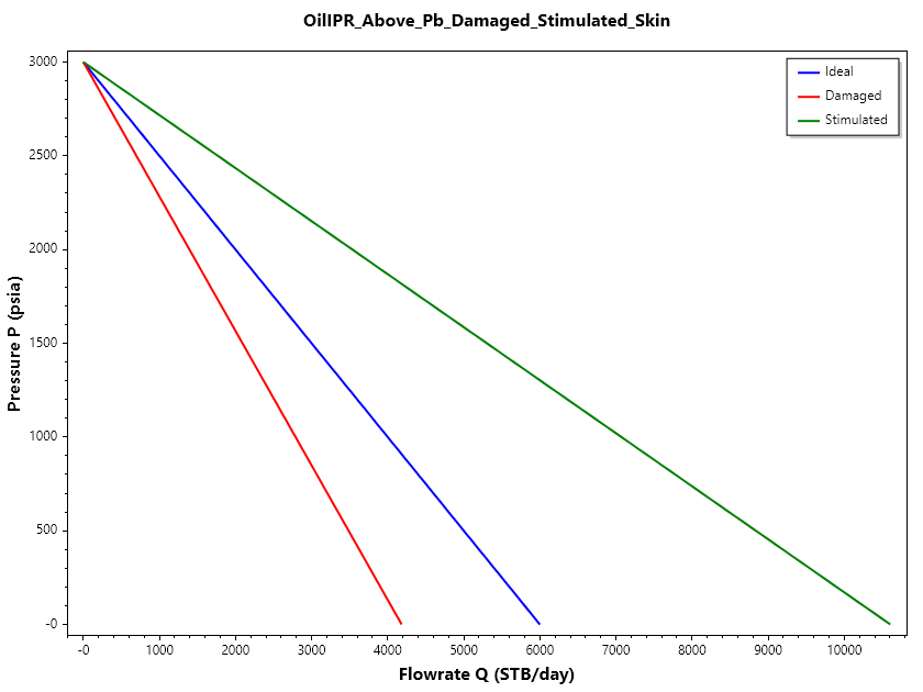
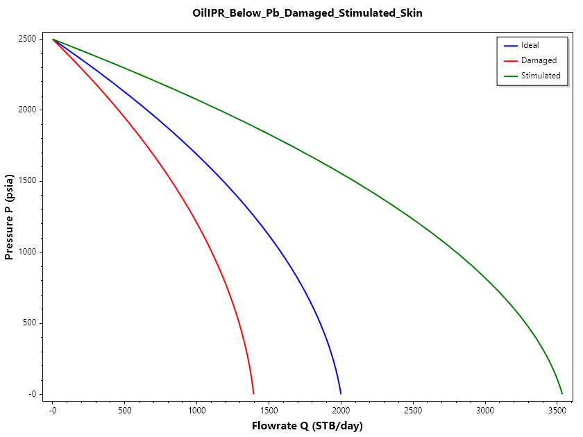
A positive skin reduces productivity, while a negative skin (stimulation) increases productivity. Numerical Example with Pressure Drop Consider a reservoir with:

$p_r = 3000 \, \text{psi}$

Bubble point pressure $p_b = 2500 \, \text{psi}$

$q_{max} = 2000 \, \text{STB/day}$

$J = 2 \, \text{STB/day/psi}$

$r_e/r_w = 1000$

$s = +3$

Case 1: Above Bubble Point ( $p_{wf} = 2800 \, \text{psi}$ )

J_s = \cfrac{2 \ln(1000)}{\ln(1000) + 3} \approx 1.3944 \\ q = 1.3944 \cdot(3000 - 2800) = 278.9 \, \text{ STB/day}

Example 4C#

double q_max = 2000; // STB/day
double p_r = 3000; // psi
double p_wf = 2800; // psi
double J = 2; // STB/day/psi
double r_e_r_w = 1000; // dimensionless
double s = 3; // dimensionless
double lnre_rw = Log(r_e_r_w);
double FE = lnre_rw/(lnre_rw + s);
double J_s = J * FE; // STB/day/psi
double q = J_s * (p_r - p_wf); // STB/day
Console.WriteLine($"Adjusted Productivity Index (J_s) = {J_s:F4} STB/day/psi");
// Full Range
double damageskin = 3;
double stimulatedskin = -3;
double FE_damage = lnre_rw/(lnre_rw + damageskin);
double FE_stimulated = lnre_rw/(lnre_rw + stimulatedskin);
double qfun(double pwf) => J * (p_r - pwf);
ColVec Prange = Linspace(0, p_r);
ColVec Qrange = Arrayfun(qfun, Prange);
Plot(Qrange, Prange, "b", 2); HoldOn();
Plot(FE_damage * Qrange, Prange, "r", 2);
Plot(FE_stimulated * Qrange, Prange, "g", 2); HoldOff();
Xlabel("Flowrate Q (STB/day)");
Ylabel("Pressure P (psia)");
Title("OilIPR_Above_Pb_Damaged_Stimulated_Skin");
Legend(["Ideal", "Damaged", "Stimulated"]);
SaveAs("OilIPR_Above_Pb_Damaged_Stimulated_Skin.png");

double q_max = 2000; // STB/day
double p_r = 3000; // psi
double p_wf = 2800; // psi
double J = 2; // STB/day/psi
double r_e_r_w = 1000; // dimensionless
double s = 3; // dimensionless
double lnre_rw = Log(r_e_r_w);
double FE = lnre_rw/(lnre_rw + s);
double J_s = J * FE; // STB/day/psi
double q = J_s * (p_r - p_wf); // STB/day
Console.WriteLine($"Adjusted Productivity Index (J_s) = {J_s:F4} STB/day/psi");

// Full Range
double damageskin = 3;
double stimulatedskin = -3;
double FE_damage = lnre_rw/(lnre_rw + damageskin);
double FE_stimulated = lnre_rw/(lnre_rw + stimulatedskin);
double qfun(double pwf) => J * (p_r - pwf);
ColVec Prange = Linspace(0, p_r);
ColVec Qrange = Arrayfun(qfun, Prange);

Plot(Qrange, Prange, "b", 2); HoldOn();
Plot(FE_damage * Qrange, Prange, "r", 2);
Plot(FE_stimulated * Qrange, Prange, "g", 2); HoldOff();
Xlabel("Flowrate Q (STB/day)");
Ylabel("Pressure P (psia)");
Title("OilIPR_Above_Pb_Damaged_Stimulated_Skin");
Legend(["Ideal", "Damaged", "Stimulated"]);
SaveAs("OilIPR_Above_Pb_Damaged_Stimulated_Skin.png");

OutputFrom the book

Adjusted Productivity Index (J_s) = 1.3944 STB/day/psi

Case 2: Below Bubble Point ( $p_{wf} = 2000 \, \text{psi}$ )

\frac{q}{2000} = 1 - 0.2 \cdot \frac{2000}{3000} - 0.8 \cdot \left(\frac{2000}{3000}\right)^2 \\ \frac{q}{ 2000} = 1 - 0.133 - 0.356 = 0.511 \\ q = 2000 \cdot 0.511 = 1022 \, \text{ STB/day}

Adjusted for skin:

q_actual = 1022 \cdot \frac{J_s}{J} = 1022 \cdot \frac{1.3944}{2} = 712.5 \, \text{STB/day}

Example 5C#

double q_max = 2000; // STB/day
double p_wf = 1000; // psi
double p_r = 2500; // psi
double J = 2;
double r_e_r_w = 1000;
double s = 3;
double lnre_rw = Log(r_e_r_w);
double FE = lnre_rw/ (lnre_rw + s);
double J_s = J * FE; // STB/day/psi
double q_ideal = q_max * (1 - 0.2 * (p_wf / p_r) - 0.8 * Pow(p_wf / p_r, 2)); // STB/day
// Full Range
double damageskin = 3;
double stimulatedskin = -3;
double FE_damage = lnre_rw/(lnre_rw + damageskin);
double FE_stimulated = lnre_rw/(lnre_rw + stimulatedskin);
double qfun(double pwf) => q_max * (1 - 0.2 * (pwf / p_r) - 0.8 * Pow(pwf / p_r, 2));
ColVec Prange = Linspace(0, p_r);
ColVec Qrange = Arrayfun(qfun, Prange);
Plot(Qrange, Prange, "b", 2); HoldOn();
Plot(FE_damage * Qrange, Prange, "r", 2);
Plot(FE_stimulated * Qrange, Prange, "g", 2); HoldOff();
Xlabel("Flowrate Q (STB/day)");
Ylabel("Pressure P (psia)");
Title("OilIPR_Below_Pb_Damaged_Stimulated_Skin");
Legend(["Ideal", "Damaged", "Stimulated"]);
SaveAs("OilIPR_Below_Pb_Damaged_Stimulated_Skin.png");

double q_max = 2000; // STB/day
double p_wf = 1000; // psi
double p_r = 2500; // psi
double J = 2;
double r_e_r_w = 1000;
double s = 3;
double lnre_rw = Log(r_e_r_w);
double FE = lnre_rw/ (lnre_rw + s);
double J_s = J * FE; // STB/day/psi
double q_ideal = q_max * (1 - 0.2 * (p_wf / p_r) - 0.8 * Pow(p_wf / p_r, 2)); // STB/day

// Full Range
double damageskin = 3;
double stimulatedskin = -3;
double FE_damage = lnre_rw/(lnre_rw + damageskin);
double FE_stimulated = lnre_rw/(lnre_rw + stimulatedskin);
double qfun(double pwf) => q_max * (1 - 0.2 * (pwf / p_r) - 0.8 * Pow(pwf / p_r, 2));
ColVec Prange = Linspace(0, p_r);
ColVec Qrange = Arrayfun(qfun, Prange);

Plot(Qrange, Prange, "b", 2); HoldOn();
Plot(FE_damage * Qrange, Prange, "r", 2);
Plot(FE_stimulated * Qrange, Prange, "g", 2); HoldOff();
Xlabel("Flowrate Q (STB/day)");
Ylabel("Pressure P (psia)");
Title("OilIPR_Below_Pb_Damaged_Stimulated_Skin");
Legend(["Ideal", "Damaged", "Stimulated"]);
SaveAs("OilIPR_Below_Pb_Damaged_Stimulated_Skin.png");

OutputFrom the book

Case 3: At Zero Bottom-Hole Pressure ( $p_{wf} = 0$ )

q = q_{max} = 2000 \, \text{STB/day}

Adjusted for skin:

q_actual = 2000 \cdot \frac{1.3944}{2} = 1394.4 \, \text{STB/day}

Example 6C#

double q_max = 2000;
double q_act = q_max * 1.3944/2;
Console.WriteLine($"Actual AOF = {q_act} STB/day");

OutputFrom the book

Actual AOF = 1394.4 STB/day

Gas Well Inflow Performance Relation (IPR)

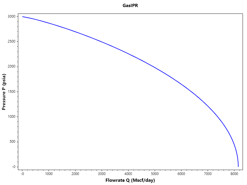
Definition: Gas Inflow Performance Relationship (IPR) describes the relationship between the gas flow rate ( $q_g$ ) and the bottom-hole flowing pressure ( $p_{wf}$ ). Unlike oil, gas productivity is highly non-linear due to the pressure-dependent properties of gas (viscosity $mu_g$ and compressibility factor $z$ ).

The Simplified Back-Pressure Equation

For most engineering applications, the Rawlins and Schellhardt empirical "Back-Pressure" equation is used to describe gas well performance:

q_g = C \cdot (p_r^2 - p_{wf}^2)^n

Where:

$q_g$ = gas flow rate (Mscf/day)

$C$ = performance coefficient (Mscf/day/psi²)

$p_r$ = average reservoir pressure (psia)

$p_{wf}$ = bottom-hole flowing pressure (psia)

$n$ = turbulence factor (typically 0.5 to 1.0)

Numerical Example:

Given:

$C = 0.01 \, \text{Mscf/day/psi}^2$

$n = 0.85$ (indicates some non-Darcy flow/turbulence)

$p_r = 3000 \, \text{psia}$

$p_{wf} = 2000 \, \text{psia}$

q_g = 0.01 \cdot (3000^2 - 2000^2)^{0.85} \\ q_g = 0.01 \cdot (5,000,000)^{0.85} \approx 4,874 , \text{Mscf/day}

Example 7C#

double C = 0.01, n = 0.85;
double p_r = 3000; // psia
double p_wf = 2000; // psia
double q_g = C * Pow(Pow(p_r, 2) - Pow(p_wf, 2), n);
Console.WriteLine($"Gas Flow Rate (q_g) = {q_g:F2} Mscf/day");
// Full Range
double qfun(double pwf) => C * Pow(Pow(p_r, 2) - Pow(pwf, 2), n);
ColVec Prange = Linspace(0, p_r);
ColVec Qrange = Arrayfun(qfun, Prange);
Plot(Qrange, Prange, "b", 2);
Xlabel("Flowrate Q (Mscf/day)");
Ylabel("Pressure P (psia)");
Title("GasIPR");
SaveAs("GasIPR.png");

OutputFrom the book

Gas Flow Rate (q_g) = 4944.52 Mscf/day

Absolute Open Flow (AOF)

The Absolute Open Flow potential is the maximum rate a well could theoretically deliver if the flowing pressure ( $p\_{wf}$ ) were reduced to zero. It is a common benchmark for gas well productivity.

AOF = C \cdot (p_r^2)^n

Numerical Example:

Using the same parameters as above:

AOF = 0.01 \cdot (3000^2)^{0.85} \\ AOF = 0.01 \cdot (9,000,000)^{0.85} \approx 8,021 \, \text{Mscf/day}

Example 8C#

double C = 0.01;
double n = 0.85;
double p_r = 3000;
double AOF = C * Pow(Pow(p_r, 2), n);
Console.WriteLine($"Absolute Open Flow (AOF) = {AOF:F2} Mscf/day");

OutputFrom the book

❌ Syntax Error in Documentation:
Line 7: Member definition, statement, or end-of-file expected

High Pressure Gas IPR (Pseudo-Pressure)

The $m(p)$ approach:/// When reservoir pressure exceeds 2000–3000 psi, the $p^2$ method becomes inaccurate. Engineers use the Real Gas Pseudo-Pressure, $m(p)$ , to linearize the flow equation:

q_g = C' \cdot [m(p_r) - m(p_{wf})]

Where:

m(p) = 2 \int_{p_{base}}^{p} \frac{p}{\mu_g z} dp

Example 9C#

// Simplified Linear Pseudo-Pressure Example
double m_pr = 6.5e8; // psi^2/cp
double m_pwf = 4.2e8; // psi^2/cp
double C_prime = 0.00002; // performance coefficient
double q_g = C_prime * (m_pr - m_pwf);
Console.WriteLine($"Pseudo-pressure Gas Rate = {q_g:F2} Mscf/day");

OutputFrom the book

Pseudo-pressure Gas Rate = 4600.00 Mscf/day

Summary of n-values:

n Value	Flow Regime	Description
n = 1.0	Fully Laminar	Darcy flow, no turbulence near wellbore.
0.5 < n < 1.0	Transitional	Common in most commercial gas wells.
n = 0.5	Fully Turbulent	High velocity flow, typical in high-rate wells.