Reineur Solver: solve real-world problems with confidence

Solution of Partial Differential Equations by Laplace Transform

The Laplace Transform is a powerful integral transform used to convert partial differential equations (PDEs) into algebraic equations, which are often easier to solve. This method is particularly useful for solving linear PDEs with constant coefficients and specific boundary conditions. While the Laplace Transform method is not a numerical methods we have decided to included it in this because of its similarity to method of lines.

1. Definition of the Laplace Transform

The Laplace Transform of a function $f(t)$ is defined as:

F(s) = \mathcal{L}\{f(t)\} = \int_{0}^{\infty} e^{-st} f(t) dt

where $s$ is a complex number frequency parameter.

2. Applying the Laplace Transform to PDEs

To solve a PDE using the Laplace Transform, we follow these steps:

Take the Laplace Transform of both sides of the PDE with respect to time variable $t$ .
Solve the resulting algebraic equation in the Laplace domain.
Apply the inverse Laplace Transform to obtain the solution in the time domain.

3. Example: Solving the Heat Equation

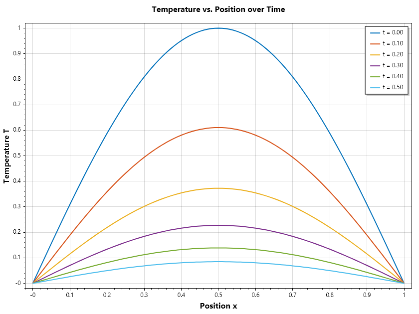
Consider the one-dimensional heat equation:

\frac{\partial u}{\partial t} = \alpha \frac{\partial^2 u}{\partial x^2}

with initial condition $u(x,0) = \sin(\pi x)$ and boundary conditions $u(0,t) = u(1,t) = 0$ .

Solution Steps:

Step 1: Take the Laplace Transform

\mathcal{L}\left\{\frac{\partial u}{\partial t}\right\} = sU(x,s) - u(x,0) = sU(x,s) - \sin(\pi x)

\mathcal{L}\left\{ \alpha \frac{\partial^2 u}{\partial x^2} \right\} = \alpha \frac{\partial^2 U}{\partial x^2}

Step 2: Transform the boundary conditions

U(0,s) = U(1,s) = 0

Step 3: Solve the Ordinary Differential Equation

sU(x,s) - \sin(\pi x) = \alpha \frac{\partial^2 U}{\partial x^2}

Rearranging gives:

\frac{\partial^2 U}{\partial x^2} - \frac{s}{\alpha}U(x,s) = -\frac{1}{\alpha}\sin(\pi x)

Homogeneous solution and particular solution methods can be applied here.

\alpha \frac{\partial^2 U}{\partial x^2} - sU(x,s) = 0

Complementary Solution:

U(x,s) = C_1(s) \sinh\left(\sqrt{\frac{s}{\alpha}}x\right) + C_2(s) \cosh\left(\sqrt{\frac{s}{\alpha}}x\right)

Particular Solution: We assume $U_p(x) = A\sin(\pi x) + B\cos(\pi x)$

by substitution in the equation we have

-\pi^2(A\sin(\pi x) + B\cos(\pi x)) - \frac{s}{\alpha} \left(A\sin(\pi x) + B\cos(\pi x) \right) = -\frac{1}{\alpha}\sin(\pi x)

it follows that $B = 0$ and $A = 1/(s + \pi^2\alpha)$

General Solution is thus:,

C_1(s) \sinh\left(\sqrt{\frac{s}{\alpha}}x\right) + C_2(s) \cosh\left(\sqrt{\frac{s}{\alpha}}x\right) + \frac{\sin(\pi x)}{s + \pi^2\alpha}

Step 4: Applying the boundary conditions:

at $x = 0$ :

U(0, s) = C_1(0) + C_2(1) + 0 = 0 \implies C_2 = 0;

at $x = 1$ :

C_1(s) \sinh\left(\sqrt{\frac{s}{\alpha}}\right) = 0 \implies C_1 = 0

hence,

U(x,s) = \frac{\sin(\pi x)}{s + \pi^2\alpha}

Step 5: Apply the inverse Laplace Transform to find $u(x,t)$

u(x, t) = \mathcal{L}^{-1}\left\{\frac{\sin(\pi x)}{ s + \pi^2\alpha} \right\} = \sin(\pi x)\mathcal{L}^{-1}\left\{ \frac{1}{s + \pi^2\alpha} \right\}

u(x, t) = e^{-\alpha\pi^2 t}\sin(\pi x)

Example 1C#

// Define the function and interval
double alpha = 0.5, π = pi;
ColVec x = Linspace(0, 1, 101);
RowVec T = Linspace(0, 0.5, 6);
Matrix U = Exp(-alpha * π * π * T).Times(Sin(π * x));
Plot(x, U, Linewidth: 2); GridOn();
Xlabel("Position x"); Ylabel("Temperature T");
Title("Temperature vs. Position over Time");
Legend(T.Select(t => $"t = {t:0.00}"));
SaveAs("Temperature_Laplace.png");

OutputFrom the book

Numerical Inversion of Laplace Transform

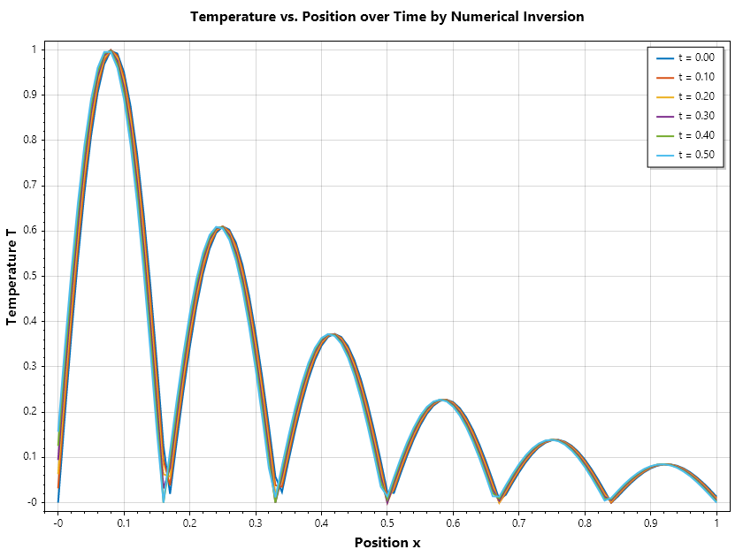
Sepalsolver has inbuilt numerical laplace transform inversion routine that allows the invesion of the solution fron Laplace space. We cn demonstrate this ability using the last example.

Example 2C#

// Define the function and interval
double alpha = 0.5, π = pi;
ColVec x = Linspace(0, 1, 101);
RowVec T = Linspace(0, 0.5, 6);
double Unuminv (double x, double t) => t == 0 ? Sin(π * x) : NiLaplace(s=> Sin(π * x)/(s + π* π*alpha), t);
Matrix U = Meshfun(Unuminv, x, T);
Plot(x, U, Linewidth: 2); GridOn();
Xlabel("Position x"); Ylabel("Temperature T");
Title("Temperature vs. Position over Time by Numerical Inversion");
Legend(T.Select(t => $"t = {t:0.00}"));
SaveAs("Temperature_Using_Numerical_Inversion_Laplace.png");

OutputFrom the book

Numerical Inversion Laplace Transform : Dimensionless Water Influx Estimation

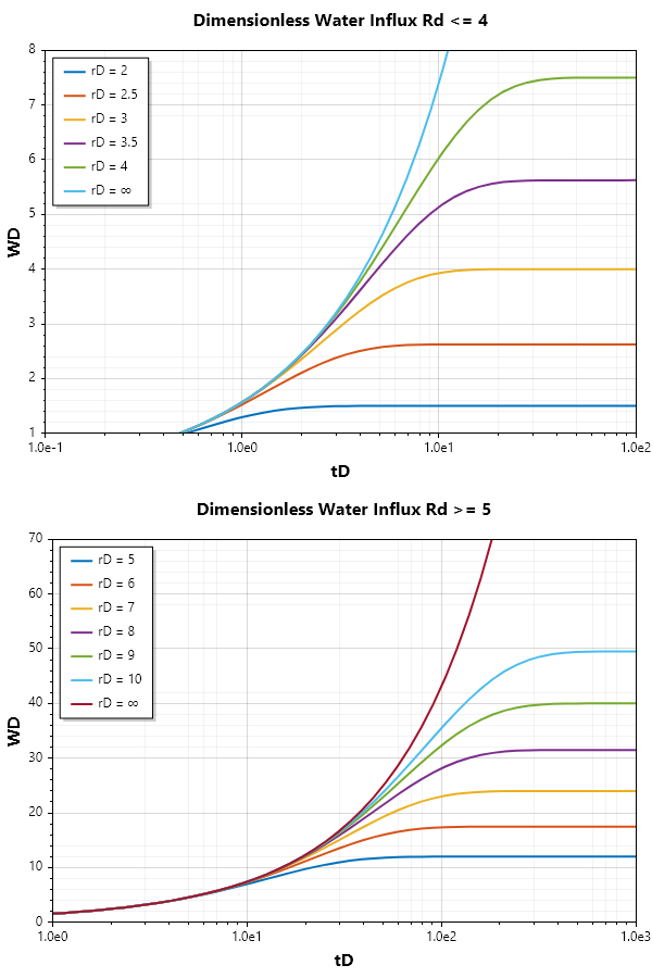
Water influx in an oil reservoir is the migration of water from an aquifer into the pore spaces of the reservoir rock containing oil. This water movement is primarily driven by pressure differences between the aquifer and the reservoir as the oil is produced and reservoir pressure declines. The water influx can provide pressure support, helping to maintain reservoir pressure and sustain oil production. Hence, understanding and accurate estimation of water influx is crucial for optimizing oil recovery strategies and the long-term economic viability of an oil field. For use in material balance computation in edge drive configuration, reservoir engneering books provide plots for Wd as a function of dimensionless radius and time

In an edge drive configuration with the aquifer closed at its outer boundary, the governing equation gives:

\cfrac{\partial P} {\partial t} = \cfrac{ 1} { r}\cfrac{\partial} {\partial r}\left(r \cfrac{\partial P} {\partial r} \right)

P(t = 0, r) = 0, P(t, r = 1) = 1, \cfrac{\partial P} {\partial r} (t, r = r_D) = 0

The solution in laplace space:

P(s, r) = \Phi_1 I_0(r\sqrt{ s}) + \Phi_2 K_0(r\sqrt{ s})

Using the boundary conditions to evaluate the constants and substitute them:

P(s, r) = \cfrac{ K_1(r_D\sqrt{ s}) I_0(r\sqrt{ s}) +I_1(r_D\sqrt{ s}) K_0(r\sqrt{ s})}{ s(K_1(r_D\sqrt{ s}) I_0(\sqrt{ s}) +I_1(r_D\sqrt{ s}) K_0(\sqrt{ s}))}

From Darcy law, we know that the rate of water influx is proportional to the negative rate of change of pressure with respect to radial position at the reservoir aquifer boundary, hence total water influx after a time t is thus:

W(t) = \int_{ 0}^{ t_D}-\cfrac{\partial P} {\partial r} (\tau, r = 1) \partial \tau

This can be accomplised by performing the integration in laplace space before inverting to time space.

W(t) = \mathcal{L}^{-1}\left(\frac{-1}{s} \cfrac{\partial P}{\partial r}(s, r = 1) \right)

W(t) = \mathcal{ L} ^{ -1}\left(\frac{ 1} { s\sqrt{ s} } \cfrac{ I_1(r_D\sqrt{ s}) K_1(\sqrt{ s}) -K_1(r_D\sqrt{ s}) I_1(\sqrt{ s})} { (I_1(r_D\sqrt{ s}) K_0(\sqrt{ s}) +K_1(r_D\sqrt{ s}) I_0(\sqrt{ s}))} \right)

Lets see how to compute water influx, and generate the started water influx plot as shown above

Example 3C#

double I0(double x) => BesselI(0, x); double I1(double x) => BesselI(1, x);
double K0(double x) => BesselK(0, x); double K1(double x) => BesselK(1, x);
// define Wd function in time space.
double EdgeClosedBoundaryRadial_Wd(double tD, double rD)
{
    double LapW(double s)
    {
        double sqrts = Sqrt(s), sqrts3 = s * sqrts;
        double Num = K1(sqrts), Den = K0(sqrts);
        if (!double.IsInfinity(rD))
        {
            double rDsqrts = rD * sqrts;
            Num = I1(rDsqrts) * Num - K1(rDsqrts) * I1(sqrts);
            Den = I1(rDsqrts) * Den + K1(rDsqrts) * I0(sqrts);
        }
        return Num / (Den * sqrts3);
    }
    return tD == 0 ? 0 : NiLaplace(LapW, tD);
}
// plotfunction 
void PlotFunction(ColVec Td, RowVec Rd)
{
    Matrix Wd = Meshfun(EdgeClosedBoundaryRadial_Wd, Td, Rd);
    SemiLogx(Td, Wd, Linewidth: 2);
    Xlabel("tD"); Ylabel("WD"); GridOn(); MinorGridOn();
    Legend(Rd.Select(rd => $"rD = {rd}"), UpperLeft);
}
{// Compute and Plot Wd for Rd <= 4
    Subplot(2, 1, 0);
    double[] Rd = [2, 2.5, 3, 3.5, 4, inf],
        Td = Logspace(-1, 2);
    PlotFunction(Td, Rd); Axis([0.1, 100, 1, 8]);
    Title("Dimensionless Water Influx Rd <= 4");
}
{// Compute and Plot Wd for Rd >= 5
    Subplot(2, 1, 1);
    double[] Rd = [5, 6, 7, 8, 9, 10, inf],
        Td = Logspace(0, 3);
    PlotFunction(Td, Rd); Axis([1, 1000, 0, 70]);
    Title("Dimensionless Water Influx Rd >= 5");
}
//Save Figure
SaveAs("Dimensionless-Water-Influx.png", 600, 900); CloseFig();
CloseFig();

double I0(double x) => BesselI(0, x); double I1(double x) => BesselI(1, x);
double K0(double x) => BesselK(0, x); double K1(double x) => BesselK(1, x);
// define Wd function in time space.
double EdgeClosedBoundaryRadial_Wd(double tD, double rD)
{
    double LapW(double s)
    {
        double sqrts = Sqrt(s), sqrts3 = s * sqrts;
        double Num = K1(sqrts), Den = K0(sqrts);
        if (!double.IsInfinity(rD))
        {
            double rDsqrts = rD * sqrts;
            Num = I1(rDsqrts) * Num - K1(rDsqrts) * I1(sqrts);
            Den = I1(rDsqrts) * Den + K1(rDsqrts) * I0(sqrts);
        }
        return Num / (Den * sqrts3);
    }
    return tD == 0 ? 0 : NiLaplace(LapW, tD);
}
// plotfunction 
void PlotFunction(ColVec Td, RowVec Rd)
{
    Matrix Wd = Meshfun(EdgeClosedBoundaryRadial_Wd, Td, Rd);
    SemiLogx(Td, Wd, Linewidth: 2);
    Xlabel("tD"); Ylabel("WD"); GridOn(); MinorGridOn();
    Legend(Rd.Select(rd => $"rD = {rd}"), UpperLeft);
}

{// Compute and Plot Wd for Rd <= 4
    Subplot(2, 1, 0);
    double[] Rd = [2, 2.5, 3, 3.5, 4, inf],
        Td = Logspace(-1, 2);
    PlotFunction(Td, Rd); Axis([0.1, 100, 1, 8]);
    Title("Dimensionless Water Influx Rd <= 4");
}

{// Compute and Plot Wd for Rd >= 5
    Subplot(2, 1, 1);
    double[] Rd = [5, 6, 7, 8, 9, 10, inf],
        Td = Logspace(0, 3);
    PlotFunction(Td, Rd); Axis([1, 1000, 0, 70]);
    Title("Dimensionless Water Influx Rd >= 5");
}

//Save Figure
SaveAs("Dimensionless-Water-Influx.png", 600, 900); CloseFig();
CloseFig();

OutputFrom the book

Takes a free account.

Solution Of PDE by Laplace Transform

Solution of Partial Differential Equations by Laplace Transform

1. Definition of the Laplace Transform

2. Applying the Laplace Transform to PDEs

3. Example: Solving the Heat Equation

Numerical Inversion of Laplace Transform

Numerical Inversion Laplace Transform : Dimensionless Water Influx Estimation