Solution Of PDE by Method of Lines — SepalSolver

The Method of Lines (MOL) is a powerful numerical technique used to solve partial differential equations (PDEs), particularly those that are time-dependent (evolutionary).

Instead of discretizing all dimensions(space and time) simultaneously, the core idea is to discretize the spatial variables while leaving the time variable continuous. This transforms a single PDE into a system of coupled Ordinary Differential Equations(ODEs).

How It Works: The 3-Step Process

Imagine you are solving the heat equation:

\frac{\partial u}{\partial t} = \alpha \frac{\partial^2 u}{\partial x^2}

Spatial Discretization: You divide the spatial domain into a grid of points(e.g., $x_1, x_2, \cdot, x_n$ ). You replace the spatial derivatives $(\frac{\partial^2 u}{\partial x^2})$ with finite difference approximations, such as:

\frac{\partial^2 u}{\partial x^2} = \frac{u_{i+1} - 2u_i + u_{i-1}}{(\Delta x)^2}

Conversion to ODEs: By applying this at every grid point, the PDE becomes a set of ODEs, one for each point :

\frac{\partial u_i(t)}{\partial t} \approx \alpha \frac{u_{i+1}(t) - 2u_i(t) + u_{i-1}(t)}{(\Delta x)^2}

Temporal Integration: Now that you have a system of ODEs, you can use standard, high-performance ODE solvers like Runge-Kutta or Euler’s method to step forward in time.

## Why Use It? (Advantages)

Leverages Existing Tech: You can use sophisticated, pre-built ODE solvers(like Ode45/Ode45a in SepalSolver or ode45 in MATLAB) that automatically handle error control and adaptive time-stepping.
Flexibility: You can use different spatial discretization methods, such as finite differences, finite elements, or spectral methods, depending on the geometry of your problem
Simplification: It breaks a complex multi-dimensional problem into a more manageable "line-by-line" temporal evolution.

## Limitations

Stiffness: The resulting system of ODEs is often "stiff," meaning you may need implicit solvers to avoid tiny, inefficient time steps.
Not for All PDEs: It is designed for "evolutionary" problems (parabolic and hyperbolic). It cannot be used directly for purely "steady-state" elliptic equations(like Laplace’s equation) without adding a "pseudo-time" variable.

Feature	Standard Finite Difference(FDM)	Method of Lines(MOL)
Time Treatment	Discretized at the start	Kept continuous initially
Solving Logic	Solves the whole grid at once	Solves ODEs along "lines" of time
Software	Requires custom time-stepping	Uses off-the-shelf ODE solvers

In sepalsolver, the nnumerical solution of pde (Pdepe) is built on Ode45a: our differential algebraic equation solver that relies on L-stable diagonally implicit Runge Kutta. This allows it to handle the boundary conditions implicitly and also correct the egde values in situation where the initial condition is not consitent with the boundary condition

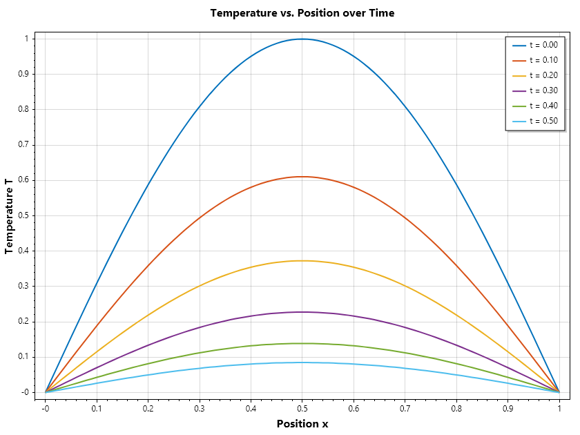
Example 1: Solving the Heat Equation

Consider the one-dimensional heat equation:

\frac{\partial u}{\partial t} = \alpha \frac{\partial^2 u}{\partial x^2}

with initial condition $u(x,0) = \sin(\pi x)$ and boundary conditions $u(0,t) = u(1,t) = 0$ .

Example 1C#

// SOLVE_HEAT_EQUATION Solves the 1D heat equation using pdepe
// Equation:  du/dt = alpha * d^2u/dx^2
// Domain:    x in [0, 1],  t in [0, 0.5]
// IC:        u(x,0) = sin(π x)
// BC:        u(0,t) = 0,  u(1,t) = 0
//
// 1. Model Parameters & Mesh Setup
double alpha = 0.5;       // Thermal diffusivity coefficient
int m = 0;                // 0 = Slab / Cartesian coordinates
double L = 1;             // Length of the rod
double t_final = 0.5;     // Final simulation time
double[] x = Linspace(0, L, 101);        // 51 spatial grid points
double[] t = Linspace(0, t_final, 6);   // 6 time steps
// 2. Defines the PDE components: c* du/ dt = x ^ (-m) * d / dx(x ^ m * f) + s
(double c, double f, double s) pdefun(double x, double t, double u, double dudx) =>
    (1, alpha * dudx, 0);
// 3. Initial sinusoidal temperature distribution
double icfun(double x) => Sin(pi * x);
// 4. Boundary Conditions defined as: p(x, t, u) + q(x, t) * f = 0
(double pl, double ql, double pr, double qr) bcfun(double xl, double ul, double xr, double ur, double t) => (ul, 0, ur, 0);
// 5. Solve the PDE
(var T, var U) = Pdepe(m, pdefun, icfun, bcfun, x, t);
// Subplot 2: 2D Temperature Profiles at Selected Times
Plot(x, U, Linewidth: 2); GridOn();
Xlabel("Position x"); Ylabel("Temperature T");
Title("Temperature vs. Position over Time");
Legend(T.Select(t => $"t = {t:0.00}"));
SaveAs("Temperature.png");
CloseFig();

// SOLVE_HEAT_EQUATION Solves the 1D heat equation using pdepe
// Equation:  du/dt = alpha * d^2u/dx^2
// Domain:    x in [0, 1],  t in [0, 0.5]
// IC:        u(x,0) = sin(π x)
// BC:        u(0,t) = 0,  u(1,t) = 0
//
// 1. Model Parameters & Mesh Setup
double alpha = 0.5;       // Thermal diffusivity coefficient
int m = 0;                // 0 = Slab / Cartesian coordinates
double L = 1;             // Length of the rod
double t_final = 0.5;     // Final simulation time

double[] x = Linspace(0, L, 101);        // 51 spatial grid points
double[] t = Linspace(0, t_final, 6);   // 6 time steps

// 2. Defines the PDE components: c* du/ dt = x ^ (-m) * d / dx(x ^ m * f) + s
(double c, double f, double s) pdefun(double x, double t, double u, double dudx) =>
    (1, alpha * dudx, 0);

// 3. Initial sinusoidal temperature distribution
double icfun(double x) => Sin(pi * x);

// 4. Boundary Conditions defined as: p(x, t, u) + q(x, t) * f = 0
(double pl, double ql, double pr, double qr) bcfun(double xl, double ul, double xr, double ur, double t) => (ul, 0, ur, 0);

// 5. Solve the PDE
(var T, var U) = Pdepe(m, pdefun, icfun, bcfun, x, t);

// Subplot 2: 2D Temperature Profiles at Selected Times
Plot(x, U, Linewidth: 2); GridOn();
Xlabel("Position x"); Ylabel("Temperature T");
Title("Temperature vs. Position over Time");
Legend(T.Select(t => $"t = {t:0.00}"));
SaveAs("Temperature.png");
CloseFig();

OutputFrom the book

Example 2: Solving Reactive Diffusion Equation

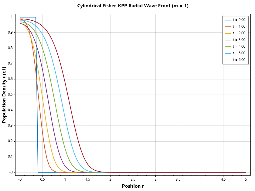
The Fisher-KPP reaction-diffusion model transformed into a cylindrical coordinate system ( $m = 1$ ). In cylindrical coordinates, the model represents radial population dispersion or chemical wavefront propagation outward from a central core (e.g., cell growth in a Petri dish or cylindrical tissue scaffold).

\frac{\partial u}{\partial t} = D\frac{1}{r}\frac{\partial}{\partial r}\left(r\frac{\partial u}{\partial r} \right) + r_g \cdot u(1 - u)

initial condition

u(r,0) = \begin{cases} 0.8 & \text{if } r < 0.5, \\ 0 & \text{otherwise} \end{cases}

boundary condition

\left.\frac{\partial u}{\partial r}\right|_{(0,t)} = 0, \quad \left.\frac{\partial u}{\partial r}\right|_{(5,t)} = 0

Example 2C#

// SOLVE-DIFFUSION-REACTION-EQUATION
// Solves the 1D reaction-diffusion equation in cylindrical coordinates using pdepe
// Equation:  du/dt = D/r*d/dr(r*du/dr) + g*u*(1 - u);
// Domain:    r in [0, 5],  t in [0, 6]
// IC:        u(r,0) = 1.0 if r < 0.4;
//                     0.0 otherwise
// BC:        du/dr(0,t) = 0,  du/dr(5,t) = 0
// 1. Model Parameters & Mesh Setup
int m = 1; // cylindrical geometry
double D = 0.01; // Diffusion coefficient
double growthRate = 1.0; // Growth rate
double[] r = Linspace(0, 5, 101);  // [0, 5]
double[] t = Linspace(0, 6, 7);    // [0, 6]
// 2. Defines the PDE components: du/dt = D/r*d/dr(r*du/dr) + g*u*(1 - u);
(double c, double f, double s) PdeFun(double r, double t, double u, double dudr)
{
    double capacity = 1.0;
    double flux = D * dudr;
    double source = growthRate * u * (1.0 - u); // Logistic reaction term
    return (capacity, flux, source);
}
// 3. Initial localized pulse at r = 0
double IcFun(double r) => r < 0.4 ? 1.0 : 0.0;
// 4. Insulated endpoints (zero flux)
(double pl, double ql, double pr, double qr) BcFun(double rl, double ul, double rr, double ur, double t)
    => (0.0, 1.0, 0.0, 1.0);
// 5. Solve the PDE
(ColVec T, Matrix U) = Pdepe(m, PdeFun, IcFun, BcFun, r, t);
Plot(r, U, Linewidth: 2); GridOn();
Title("Cylindrical Fisher-KPP Radial Wave Front (m = 1)");
Xlabel("Position r"); Ylabel("Population Density u(r,t)");
Legend(T.Select(t => $"t = {t:0.00}"));
SaveAs("Cylindrical_FisherKPP.png");
CloseFig();

// SOLVE-DIFFUSION-REACTION-EQUATION
// Solves the 1D reaction-diffusion equation in cylindrical coordinates using pdepe
// Equation:  du/dt = D/r*d/dr(r*du/dr) + g*u*(1 - u);
// Domain:    r in [0, 5],  t in [0, 6]
// IC:        u(r,0) = 1.0 if r < 0.4;
//                     0.0 otherwise
// BC:        du/dr(0,t) = 0,  du/dr(5,t) = 0

// 1. Model Parameters & Mesh Setup
int m = 1; // cylindrical geometry
double D = 0.01; // Diffusion coefficient
double growthRate = 1.0; // Growth rate
double[] r = Linspace(0, 5, 101);  // [0, 5]
double[] t = Linspace(0, 6, 7);    // [0, 6]

// 2. Defines the PDE components: du/dt = D/r*d/dr(r*du/dr) + g*u*(1 - u);
(double c, double f, double s) PdeFun(double r, double t, double u, double dudr)
{
    double capacity = 1.0;
    double flux = D * dudr;
    double source = growthRate * u * (1.0 - u); // Logistic reaction term
    return (capacity, flux, source);
}

// 3. Initial localized pulse at r = 0
double IcFun(double r) => r < 0.4 ? 1.0 : 0.0;

// 4. Insulated endpoints (zero flux)
(double pl, double ql, double pr, double qr) BcFun(double rl, double ul, double rr, double ur, double t)
    => (0.0, 1.0, 0.0, 1.0);

// 5. Solve the PDE
(ColVec T, Matrix U) = Pdepe(m, PdeFun, IcFun, BcFun, r, t);

Plot(r, U, Linewidth: 2); GridOn();
Title("Cylindrical Fisher-KPP Radial Wave Front (m = 1)");
Xlabel("Position r"); Ylabel("Population Density u(r,t)");
Legend(T.Select(t => $"t = {t:0.00}"));
SaveAs("Cylindrical_FisherKPP.png");
CloseFig();

OutputFrom the book

It is important to note that pdepe can be invoked with a shothand form as shown in the example below

Example 3C#

double D = 0.01;                  // Diffusion coefficient
double growthRate = 1.0;          // Growth rate
double C_ambient = 0.0;           // Ambient/Boundary concentration
double[] r = Linspace(0, 5, 101); // Spatial grid [0, 5]
double[] t = Linspace(0, 6, 7);   // Time output points [0, 6]
(ColVec T, Matrix U) = Pdepe(
    m: 1,                                                                     // Geometry: 0 = Cartesian, 1 = Cylindrical, 2 = Spherical
    pdefun: (r, t, u, dudr) => (1.0, D * dudr, growthRate * u * (1.0 - u)),   // PDE components: (c, f, s) -> du/dt = D/r*d/dr(r*du/dr) + g*u*(1-u)
    icfun: r => r < 0.4 ? 1.0 : 0.0,                                          // Initial condition: u(r,0) = 1 for r < 0.4, else 0
    bcfun: (rl, ul, rr, ur, t) => (0, 1, ur - C_ambient, 0),                  // BCs: Symmetry at origin (du/dr = 0), Dirichlet at boundary (u(5,t) = C_ambient)
    x: r,                                                                     // Spatial discretization array
    t: t);                                                                    // Solution output times
Plot(r, U, Linewidth: 2); GridOn();
Title("Cylindrical Fisher-KPP Radial Wave Front (m = 1)");
Xlabel("Position r"); Ylabel("Population Density u(r,t)");
Legend(T.Select(time => $"t = {time:0.00}"));
SaveAs("Cylindrical_FisherKPP.png");
CloseFig();

double D = 0.01;                  // Diffusion coefficient
double growthRate = 1.0;          // Growth rate
double C_ambient = 0.0;           // Ambient/Boundary concentration

double[] r = Linspace(0, 5, 101); // Spatial grid [0, 5]
double[] t = Linspace(0, 6, 7);   // Time output points [0, 6]

(ColVec T, Matrix U) = Pdepe(
    m: 1,                                                                     // Geometry: 0 = Cartesian, 1 = Cylindrical, 2 = Spherical
    pdefun: (r, t, u, dudr) => (1.0, D * dudr, growthRate * u * (1.0 - u)),   // PDE components: (c, f, s) -> du/dt = D/r*d/dr(r*du/dr) + g*u*(1-u)
    icfun: r => r < 0.4 ? 1.0 : 0.0,                                          // Initial condition: u(r,0) = 1 for r < 0.4, else 0
    bcfun: (rl, ul, rr, ur, t) => (0, 1, ur - C_ambient, 0),                  // BCs: Symmetry at origin (du/dr = 0), Dirichlet at boundary (u(5,t) = C_ambient)
    x: r,                                                                     // Spatial discretization array
    t: t);                                                                    // Solution output times

Plot(r, U, Linewidth: 2); GridOn();
Title("Cylindrical Fisher-KPP Radial Wave Front (m = 1)");
Xlabel("Position r"); Ylabel("Population Density u(r,t)");
Legend(T.Select(time => $"t = {time:0.00}"));
SaveAs("Cylindrical_FisherKPP.png");
CloseFig();

Example 3: System of Partial Differential Equations

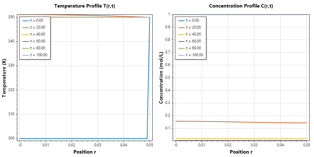
Here is a classic engineering problem: Coupled Transient Heat and Mass Transfer in a Cylindrical Reactor / Packed Bed (with $m = 1$ ). This models fluid flowing axially through a cylindrical pipe where a chemical reaction occurs, generating heat and consuming reactant along both the radial direction $r$ and over time $t$ .

Governing System of Equations For radial coordinate $r \in [r_0, R]$ (or $x \in [0, R]$ ) and time $t > 0$ , we track two coupled variables:

Temperature $T(r,t)$
Reactant Concentration $C(r,t)$

\begin{aligned} \rho C_p \frac{\partial T}{\partial t} &= \frac{1}{r} \frac{\partial}{\partial r} \left( r \cdot k \frac{\partial T}{\partial r} \right) + (-\Delta H) \cdot k_0 C e^{-\frac{E_a}{R_g T}} \\ \frac{\partial C}{\partial t} &= \frac{1}{r} \frac{\partial}{\partial r} \left( r \cdot D \frac{\partial C}{\partial r} \right) - k_0 C e^{-\frac{E_a}{R_g T}} \end{aligned}

Standard Pdepe Vector Mapping

In terms of the pdepe flux-source balance equation with cylindrical symmetry ( $m = 1$ ):

c\left(x,t,\mathbf{u},\frac{\partial \mathbf{u}}{\partial x}\right) \frac{\partial \mathbf{u}}{\partial t} = x^{-1} \frac{\partial}{\partial x}\left(x^1 \mathbf{f}\left(x,t,\mathbf{u},\frac{\partial \mathbf{u}}{\partial x}\right)\right) + \mathbf{s}\left(x,t,\mathbf{u},\frac{\partial \mathbf{u}}{\partial x}\right)

We map state vector $\mathbf{u} = \begin{bmatrix} T \\ C \end{bmatrix}$ (where $u_1 = T$ , $u_2 = C$ and spatial coordinate $x = r$ ):

-Capacities $\mathbf{c}$ :

c = \begin{bmatrix} \rho C_p \\ 1 \end{bmatrix}

Fluxes $\mathbf{f}$ :

f = \begin{bmatrix} k \frac{\partial T}{\partial r} \\ D \frac{\partial C}{\partial r} \end{bmatrix}

Sources $\mathbf{s}$ :

s = \begin{bmatrix} (-\Delta H) \cdot k_0 C e^{-\frac{E_a}{R_g T}} \\ -k_0 C e^{-\frac{E_a}{R_g T}} \end{bmatrix}

Example 4C#

// System Parameters
double rho = 1000.0;    // Density
double Cp = 4.184;      // Heat capacity
double k = 0.6;         // Thermal conductivity
double D = 1.0e-5;      // Diffusivity
double dH = -50000.0;   // Heat of reaction (exothermic)
double k0 = 100.0;      // Reaction rate constant
double Ea = 20000.0;    // Activation energy
double Rg = 8.314;      // Gas constant
// 1. PDE Definition
(ColVec c, ColVec f, ColVec s) PdeFun(double r, double t, ColVec u, ColVec dudr)
{
    double T = u[0], C = u[1];
    double dTdr = dudr[0], dCdr = dudr[1];
    // Reaction rate term
    double rate = k0 * C * Exp(-Ea / (Rg * T));
    double[] cVec = [rho * Cp, 1.0],  fVec = [k * dTdr, D * dCdr], sVec = [-dH * rate, -rate];
    return (cVec, fVec, sVec);
}
// 2. Initial Conditions (T0 = 300K, C0 = 1.0 mol/L)
ColVec IcFun(double r)
{
    double[] ic =  [300.0, 1.0];
    return ic;
}
// 3. Boundary Conditions
// At r = 0 (Symmetry): Zero flux for both T and C -> f(0,t) = 0
// At r = R (Cylindrical wall): Constant wall temp Tw, zero mass flux
(ColVec pl, ColVec ql, ColVec pr, ColVec qr) BcFun(double rLeft, ColVec uLeft, double rRight, ColVec uRight, double t)
{
    double Tw = 350.0; // Cooling/heating wall temperature
    // Left Boundary (r = 0, Symmetry) -> 0 + 1*f = 0
    double[] pl = [0.0, 0.0], ql = [1.0, 1.0];
    // Right Boundary (r = R) -> Dirichlet for T, Neumann (Zero flux) for C
    double[] pr = [uRight[0] - Tw, 0.0], qr = [0.0, 1.0];
    return (pl, ql, pr, qr);
}
// 4. Execution Call
int m = 1; // Cylindrical coordinates
double[] rMesh = Linspace(0.0, 0.05, 51); // Cylinder radius = 5 cm
double[] tMesh = Linspace(0.0, 100.0, 6);
// Solves and returns Ys[0] for T(r,t) and Ys[1] for C(r,t)
(ColVec t, Matrix[] Ys) = Pdepe(m, PdeFun, IcFun, BcFun, rMesh, tMesh);
Matrix T_sol = Ys[0]; // [TimeSteps x SpatialNodes] for Temperature
Matrix C_sol = Ys[1]; // [TimeSteps x SpatialNodes] for Concentration
Subplot(1, 2, 0);
Plot(rMesh, T_sol, Linewidth: 2); GridOn();
Title("Temperature Profile T(r,t)");
Xlabel("Position r"); Ylabel("Temperature (K)");
Legend(t.Select(t => $"t = {t:0.00}"), UpperLeft);
Subplot(1, 2, 1);
Plot(rMesh, C_sol, Linewidth: 2); GridOn();
Title("Concentration Profile C(r,t)");
Xlabel("Position r"); Ylabel("Concentration (mol/L)");
Legend(t.Select(t => $"t = {t:0.00}"), UpperLeft);
SaveAs("System_of_PDE.png");
CloseFig();

// System Parameters
double rho = 1000.0;    // Density
double Cp = 4.184;      // Heat capacity
double k = 0.6;         // Thermal conductivity
double D = 1.0e-5;      // Diffusivity
double dH = -50000.0;   // Heat of reaction (exothermic)
double k0 = 100.0;      // Reaction rate constant
double Ea = 20000.0;    // Activation energy
double Rg = 8.314;      // Gas constant

// 1. PDE Definition
(ColVec c, ColVec f, ColVec s) PdeFun(double r, double t, ColVec u, ColVec dudr)
{
    double T = u[0], C = u[1];
    double dTdr = dudr[0], dCdr = dudr[1];

// Reaction rate term
    double rate = k0 * C * Exp(-Ea / (Rg * T));
    double[] cVec = [rho * Cp, 1.0],  fVec = [k * dTdr, D * dCdr], sVec = [-dH * rate, -rate];

return (cVec, fVec, sVec);
}

// 2. Initial Conditions (T0 = 300K, C0 = 1.0 mol/L)
ColVec IcFun(double r)
{
    double[] ic =  [300.0, 1.0];
    return ic;
}

// 3. Boundary Conditions
// At r = 0 (Symmetry): Zero flux for both T and C -> f(0,t) = 0
// At r = R (Cylindrical wall): Constant wall temp Tw, zero mass flux
(ColVec pl, ColVec ql, ColVec pr, ColVec qr) BcFun(double rLeft, ColVec uLeft, double rRight, ColVec uRight, double t)
{
    double Tw = 350.0; // Cooling/heating wall temperature

// Left Boundary (r = 0, Symmetry) -> 0 + 1*f = 0
    double[] pl = [0.0, 0.0], ql = [1.0, 1.0];

// Right Boundary (r = R) -> Dirichlet for T, Neumann (Zero flux) for C
    double[] pr = [uRight[0] - Tw, 0.0], qr = [0.0, 1.0];

return (pl, ql, pr, qr);
}

// 4. Execution Call
int m = 1; // Cylindrical coordinates
double[] rMesh = Linspace(0.0, 0.05, 51); // Cylinder radius = 5 cm
double[] tMesh = Linspace(0.0, 100.0, 6);

// Solves and returns Ys[0] for T(r,t) and Ys[1] for C(r,t)
(ColVec t, Matrix[] Ys) = Pdepe(m, PdeFun, IcFun, BcFun, rMesh, tMesh);

Matrix T_sol = Ys[0]; // [TimeSteps x SpatialNodes] for Temperature
Matrix C_sol = Ys[1]; // [TimeSteps x SpatialNodes] for Concentration

Subplot(1, 2, 0);
Plot(rMesh, T_sol, Linewidth: 2); GridOn();
Title("Temperature Profile T(r,t)");
Xlabel("Position r"); Ylabel("Temperature (K)");
Legend(t.Select(t => $"t = {t:0.00}"), UpperLeft);

Subplot(1, 2, 1);
Plot(rMesh, C_sol, Linewidth: 2); GridOn();
Title("Concentration Profile C(r,t)");
Xlabel("Position r"); Ylabel("Concentration (mol/L)");
Legend(t.Select(t => $"t = {t:0.00}"), UpperLeft);
SaveAs("System_of_PDE.png");
CloseFig();

OutputFrom the book

Example 4: Higher Order in time: Wave Equation 1D

This is haneld using the system of PDE just like we use system of ode to handle higher oder odes. We first convert the higher oder derivative in time to system of first order time pdes.

Lets look as example of a string fixed at the right end and exited at the left end according to $0.5 Sin(10*t)$ .

\frac{\partial^2 u}{\partial t^2} = c^2\frac{\partial^2 u}{\partial x^2}

initial condition

u(x,0) = 0

boundary condition

u(0, t) = 0.5\sin(20t)

u(L, t) = 0

To solve this, we set $v = \cfrac{\partial u}{\partial t}$ This means we also have to differentiate the boundary conditions. And then we have

\begin{align} \frac{\partial u}{\partial t} = v \\ \frac{\partial v}{\partial t} = c^2\frac{\partial^2 u}{\partial x^2} \end{align}

initial condition

\begin{align} u(x,0) = 0\\ v(x,0) = 0 \end{align}

boundary condition

\begin{align} u(0, t) = 0.5\sin(20t)\\ v(0, t) = 10\cos(20t) \end{align}

\begin{align} u(L, t) = 0\\ v(L, t) = 0 \end{align}

Example 5C#

// 1. PDE Definition
(ColVec c, ColVec f, ColVec s) PdeFun(double r, double t, ColVec u, ColVec dudx)
{
    double V = u[1], dUdx = dudx[0];
    double[] cVec = [1, 1], fVec = [0, dUdx], sVec = [V, 0];
    return (cVec, fVec, sVec);
}
// 2. Initial Conditions (T0 = 300K, C0 = 1.0 mol/L)
ColVec IcFun(double r)
{
    double[] ic = [0, 0];
    return ic;
}
// 3. Boundary Conditions
// At r = 0 (Symmetry): Zero flux for both T and C -> f(0,t) = 0
// At r = R (Cylindrical wall): Constant wall temp Tw, zero mass flux
(ColVec pl, ColVec ql, ColVec pr, ColVec qr) BcFun(double rLeft, ColVec uLeft, double rRight, ColVec uRight, double t)
{
    // Left Boundary (x = 0) -> u-0.5*sin(20t) = 0
    double[] pl = [uLeft[0] - 0.5 * Sin(20 * t), uLeft[1] - 10 * Cos(20 * t)],
             ql = [0.0, 0.0];
    // Right Boundary (x = L) -> Fixed: Dirichlet for U and V, 
    double[] pr = [uRight[0], uRight[1]],  qr = [0.0, 0.0];
    return (pl, ql, pr, qr);
}
// 4. Execution Call
int m = 0; // Cartesian coordinates
double[] x = Linspace(0, 1, 101);
double[] t = Linspace(0, 2, 101);
(ColVec T, Matrix[] Ys) = Pdepe(m, PdeFun, IcFun, BcFun, x, t);
Matrix U = Ys[0]; // [TimeSteps x SpatialNodes] for Position
Matrix V = Ys[1]; // [TimeSteps x SpatialNodes] for Velocity
var wave = Plot(x, U[0, ..], Linewidth: 2);
Axis([x[0], x[^1], -5, 5]);
// Animation
byte[] Animfun(int i)
{
    wave.Ydata = U[i, ..].T;
    return GetFrame();
}
AnimationMaker(Animfun, "Wave_Equation_Using_PDEPE.gif", 10, T.Numel);
CloseFig();

// 1. PDE Definition
(ColVec c, ColVec f, ColVec s) PdeFun(double r, double t, ColVec u, ColVec dudx)
{
    double V = u[1], dUdx = dudx[0];
    double[] cVec = [1, 1], fVec = [0, dUdx], sVec = [V, 0];
    return (cVec, fVec, sVec);
}

// 2. Initial Conditions (T0 = 300K, C0 = 1.0 mol/L)
ColVec IcFun(double r)
{
    double[] ic = [0, 0];
    return ic;
}

// 3. Boundary Conditions
// At r = 0 (Symmetry): Zero flux for both T and C -> f(0,t) = 0
// At r = R (Cylindrical wall): Constant wall temp Tw, zero mass flux
(ColVec pl, ColVec ql, ColVec pr, ColVec qr) BcFun(double rLeft, ColVec uLeft, double rRight, ColVec uRight, double t)
{
    // Left Boundary (x = 0) -> u-0.5*sin(20t) = 0
    double[] pl = [uLeft[0] - 0.5 * Sin(20 * t), uLeft[1] - 10 * Cos(20 * t)],
             ql = [0.0, 0.0];

// Right Boundary (x = L) -> Fixed: Dirichlet for U and V, 
    double[] pr = [uRight[0], uRight[1]],  qr = [0.0, 0.0];

return (pl, ql, pr, qr);
}

// 4. Execution Call
int m = 0; // Cartesian coordinates
double[] x = Linspace(0, 1, 101);
double[] t = Linspace(0, 2, 101);

(ColVec T, Matrix[] Ys) = Pdepe(m, PdeFun, IcFun, BcFun, x, t);

Matrix U = Ys[0]; // [TimeSteps x SpatialNodes] for Position
Matrix V = Ys[1]; // [TimeSteps x SpatialNodes] for Velocity

var wave = Plot(x, U[0, ..], Linewidth: 2);
Axis([x[0], x[^1], -5, 5]);
// Animation
byte[] Animfun(int i)
{
    wave.Ydata = U[i, ..].T;
    return GetFrame();
}
AnimationMaker(Animfun, "Wave_Equation_Using_PDEPE.gif", 10, T.Numel);
CloseFig();

Example 5: Higher Dimension: Wave Equation Example

For higher dimensions, the same method can be applied. This will be demonstrated using wave equation assume $c > 0$

\frac{\partial^2 u}{\partial t^2} = c^2\left(\frac{\partial^2 u}{\partial x^2} + \frac{\partial^2 u}{\partial y^2} \right)

initial condition

u(x,y,0) = \begin{cases} 0.5\left(1 + \cos\left(\cfrac{\pi r(x, y)}{R} \right) \right) & \text{if } r(x,y) < R, \\ 0 & \text{otherwise} \end{cases}

where $r = \sqrt{(x - x_c)^2 + (y - y_c)^2}$

boundary condition

u(\pm L/2, y, t) = 0~\text{for}~y \in [-L/2, L/2]

u(x, \pm L/2, t) = 0~\text{for}~x \in [-L/2, L/2]

Step 1: Convert to system of first order PDEs in time

\frac{\partial u}{\partial t} = v

and hence

\frac{\partial v}{\partial t} = c^2\left(\frac{\partial^2 u}{\partial x^2} + \frac{\partial^2 u}{\partial y^2} \right)

Step 2: discretize the spatial part of the equation as:

\frac{\partial^2 u}{\partial x^2} = \frac{u(i+1, j) - 2u(i, j) + u(i-1, j)}{(\Delta x)^2}

\frac{\partial^2 u}{\partial y^2} = \frac{u(i, j+1) - 2u(i, j) + u(i, j-1)}{(\Delta y)^2}

Step 3: Assemble the system of coupled ODEs

\frac{\partial u(i, j)}{\partial t} = v(i, j)

\frac{\partial v(i, j)}{\partial t} = c^2\left(\frac{u(i+1, j) - 2u(i, j) + u(i-1, j)}{(\Delta x)^2} + \frac{u(i, j+1) - 2u(i, j) + u(i, j-1)}{(\Delta y)^2} \right)

We were given boundary conditions for u but we introduce v, so we have to create the boubdary condition for that by differentiating the given boundary condition.

\frac{\partial u}{\partial t}(\pm L/2, y, t) = 0~\text{for}~y \in [-L/2, L/2]

\frac{\partial u}{\partial t}(x, \pm L/2, t) = 0~\text{for}~x \in [-L/2, L/2]

we can do so for $\partial u/\partial t$ too

\frac{\partial v}{\partial t}(\pm L/2, y, t) = 0~\text{for}~y \in [-L/2, L/2]

\frac{\partial v}{\partial t}(x, \pm L/2, t) = 0~\text{for}~x \in [-L/2, L/2]

Example 6C#

// Set the domain
int Nx = 100, Ny = 100;
double Lx = 1, Ly = 1;
double c = 1, dx = Lx / Nx, dy = Ly / Ny;
double[] x = Linspace(-Lx / 2, Lx / 2, Nx + 1);
double[] y = Linspace(-Ly / 2, Ly / 2, Ny + 1);
(var X, var Y) = Meshgrid(x, y);
// Compute dt to ensure the solution is stable
double CFL = 0.3;
double dt = CFL * (dx * dy) / (c * Hypot(dx, dy));
double dx2 = dx * dx, dy2 = dy * dy, c2 = c * c;
// Set the function the computes the derivatives
(Matrix du, Matrix dv) duvdt(Matrix u, Matrix v)
{
    Matrix du = v, dv = Zeros(Nx + 1, Ny + 1);
    Matrix d2udx2 = (u[..^2, 1..^1] - 2 * u[1..^1, 1..^1] + u[2.., 1..^1]) / dx2;
    Matrix d2udy2 = (u[1..^1, ..^2] - 2 * u[1..^1, 1..^1] + u[1..^1, 2..]) / dy2;
    dv[1..^1, 1..^1] = c2 * (d2udx2 + d2udy2);
    return (du, dv);
}
// RungeKutta Integrator
(Matrix u, Matrix v) rk4(Matrix u, Matrix v)
{
    (var ku1, var kv1) = duvdt(u, v);
    (var ku2, var kv2) = duvdt(u + 0.5 * ku1 * dt, v + 0.5 * kv1 * dt);
    (var ku3, var kv3) = duvdt(u + 0.5 * ku2 * dt, v + 0.5 * kv2 * dt);
    (var ku4, var kv4) = duvdt(u + ku3 * dt, v + kv3 * dt);
    u += (ku1 + 2 * ku2 + 2 * ku3 + ku4) * dt / 6;
    v += (kv1 + 2 * kv2 + 2 * kv3 + kv4) * dt / 6;
    return (u, v);
}
// Initialize
double xc = 0, yc = -0.4, R = 0.1;
Matrix r = Hypot(X - xc, Y - yc);
Matrix U = 1 + Cos(pi * r / R), V = Zeros(Nx + 1, Ny + 1);
U[r > R] = 0;
// Simulate
int n = 1;
while (n < 1000)
{
    (U, V) = rk4(U, V);
    n++;
}

// Set the domain
int Nx = 100, Ny = 100;
double Lx = 1, Ly = 1;
double c = 1, dx = Lx / Nx, dy = Ly / Ny;
double[] x = Linspace(-Lx / 2, Lx / 2, Nx + 1);
double[] y = Linspace(-Ly / 2, Ly / 2, Ny + 1);
(var X, var Y) = Meshgrid(x, y);

// Compute dt to ensure the solution is stable
double CFL = 0.3;
double dt = CFL * (dx * dy) / (c * Hypot(dx, dy));
double dx2 = dx * dx, dy2 = dy * dy, c2 = c * c;

// Set the function the computes the derivatives
(Matrix du, Matrix dv) duvdt(Matrix u, Matrix v)
{
    Matrix du = v, dv = Zeros(Nx + 1, Ny + 1);
    Matrix d2udx2 = (u[..^2, 1..^1] - 2 * u[1..^1, 1..^1] + u[2.., 1..^1]) / dx2;
    Matrix d2udy2 = (u[1..^1, ..^2] - 2 * u[1..^1, 1..^1] + u[1..^1, 2..]) / dy2;
    dv[1..^1, 1..^1] = c2 * (d2udx2 + d2udy2);
    return (du, dv);
}

// RungeKutta Integrator
(Matrix u, Matrix v) rk4(Matrix u, Matrix v)
{
    (var ku1, var kv1) = duvdt(u, v);
    (var ku2, var kv2) = duvdt(u + 0.5 * ku1 * dt, v + 0.5 * kv1 * dt);
    (var ku3, var kv3) = duvdt(u + 0.5 * ku2 * dt, v + 0.5 * kv2 * dt);
    (var ku4, var kv4) = duvdt(u + ku3 * dt, v + kv3 * dt);
    u += (ku1 + 2 * ku2 + 2 * ku3 + ku4) * dt / 6;
    v += (kv1 + 2 * kv2 + 2 * kv3 + kv4) * dt / 6;
    return (u, v);
}

// Initialize
double xc = 0, yc = -0.4, R = 0.1;
Matrix r = Hypot(X - xc, Y - yc);
Matrix U = 1 + Cos(pi * r / R), V = Zeros(Nx + 1, Ny + 1);
U[r > R] = 0;

// Simulate
int n = 1;
while (n < 1000)
{
    (U, V) = rk4(U, V);
    n++;
}