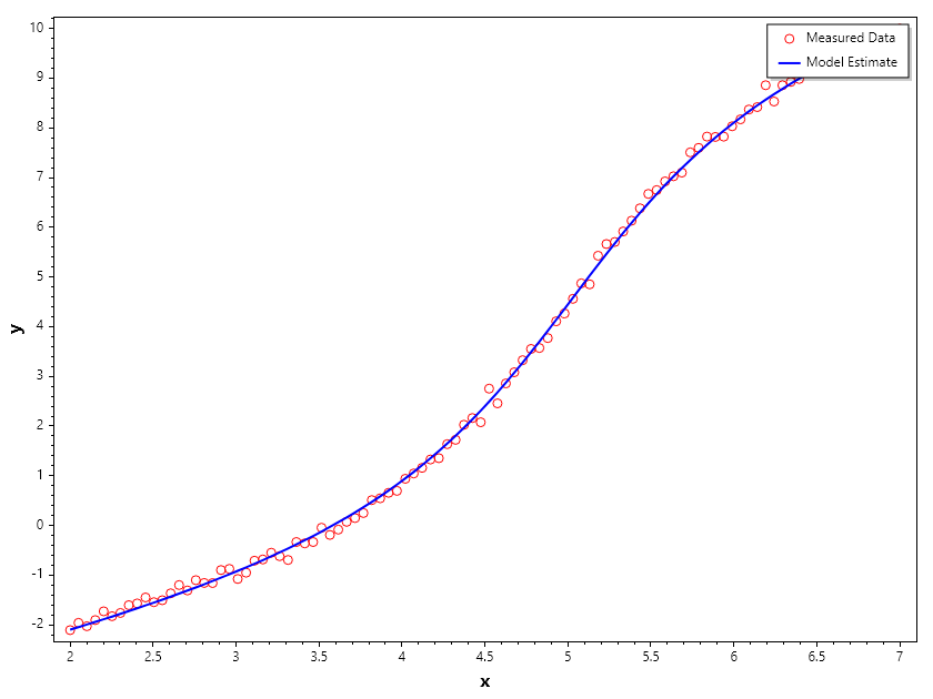
Curve Fitting

Curve fitting is a mathematical technique used to construct a curve that best fits a series of data points. It is widely applied in data analysis, statistics, and machine learning to model relationships between variables.

Types of Curve Fitting:

Linear Regression: Fits a straight line to the data points.
Polynomial Regression: Fits a polynomial curve of degree n to the data points.
Nonlinear Regression: Fits a nonlinear model to the data points.

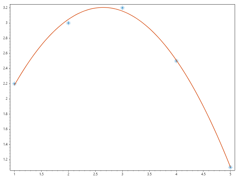
Example: Polynomial Curve Fitting

Given a set of data points, we can fit a polynomial curve using least squares optimization.

\min_{\mathbf{p}} \sum_{i=1}^{n} (y_i - P(x_i; \mathbf{p}))^2

Example 1C#

// Sample data points
double[] xData = [1, 2, 3, 4, 5];
double[] yData = [2.2, 3.0, 3.2, 2.5, 1.1];
// Fit a polynomial of degree 2
int degree = 2;
var coefficients = Polyfit(xData, yData, degree);
Scatter(xData, yData, "*", 15); HoldOn();
// Generate fitted curve
double[] xFit = Linspace(1, 5, 100);
double[] yFit = Polyval(coefficients, xFit);
Plot(xFit, yFit, Linewidth: 2);
SaveAs("Polynomial_Fitting.png");
CloseFig();

OutputFrom the book

Example: Fourier Series Fitting

Evaluating a Fourier series numerically involves transforming an infinite sum of trigonometric terms into a computationally stable, finite calculation while controlling truncation errors, floating-point precision loss, and spectral artifacts.

Mathematical Formulation:

A truncated Fourier series approximating a periodic function $f(x)$ on the interval $[-\pi, \pi]$ with $N$ harmonics is defined as:

f_N(x) = \frac{a_0}{2} + \sum_{n=1}^{N} \left( a_n \cos(nx) + b_n \sin(nx) \right)

In complex exponential form, which is computationally convenient for many numerical implementations, the series is expressed as:

f_N(x) = \sum_{n=-N}^{N} c_n e^{i n x}

where the complex coefficients $c_n$ relate to the real coefficients via:

c_0 = \frac{a_0}{2}, \quad c_n = \frac{a_n - i b_n}{2}, \quad c_{-n} = \frac{a_n + i b_n}{2}

Example 2C#

ColVec x = Linspace(-10, 10, 1001);
ColVec Rect = Sign(Sin(x));
Plot(x, Rect, Linewidth: 2); HoldOn();
var fourier = Plot(x, 0 * x, "r", Linewidth: 2);
Axis([x[0], x[^1], -1.5, 1.5]);
byte[] Animfun(int N)
{
    Matrix A = Zeros(1001, 2 * N + 3);
    A[.., 0] = Ones(1001);
    for (int n = 1; n <= (N + 1); n++)
    {
        A[.., 2 * n-1] = Cos(n * x); 
        A[.., 2 * n] = Sin(n * x);
    }
    ColVec p = Mldivide(A, Rect);
    fourier.Ydata = A * p;
    return GetFrame();
}
AnimationMaker(Animfun, "FourierFitting.gif", 5, 100);
CloseFig();

Example: Bi-Exponential Curve Fitting

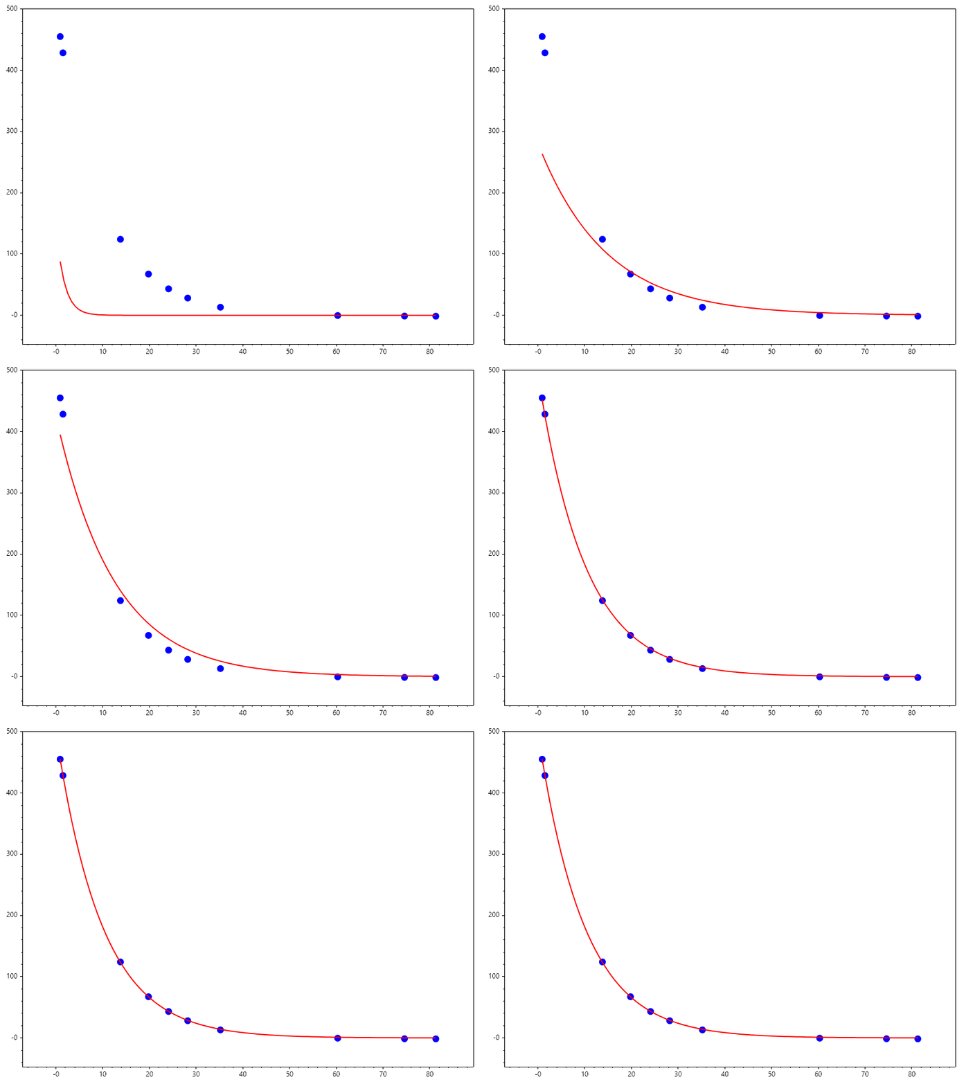
This exercise covers non-linear parameter estimation using least-squares optimization to fit a bi-exponential model to noisy data while visualizing optimizer convergence.

The objective is to fit data points $(x_d, y_d)$ to a bi - exponential model:

f(x; \theta) = \theta_2 e^{\theta_0 x} + \theta_3 e^{\theta_1 x}

where math:\theta = [\theta_0, \theta_1, \theta_2, \theta_3]^T represents the unknown parameters.

Find $\hat{\theta}$ minimizing the sum of squared residuals:

\hat{\theta} = \arg\min_{\theta} \sum_{d=1}^D (y_d - f(x_d; \theta))^2

Example 3C#

ColVec noise, weight = new double[100]; double[] x0;
static ColVec fun(ColVec x, ColVec xdata) => x[2] * Exp(x[0] * xdata) + x[3] * Exp(x[1] * xdata);
ColVec xdata = Linspace(0, 1); noise = Rand(xdata.Numel);
ColVec ydata = fun(x0 = [-4, -5, 4, -4], xdata) + 0.02 * noise;
x0 = [-1, -2, 1, -1]; weight[xdata < 0.5] = 1;
var opts = OptimSet(Display: true, MaxIter: 200, StepTol: 1e-6, OptimalityTol: 1e-6);
var ans = Lsqcurvefit(fun, x0, xdata, ydata, options: opts);
AnimateHistory(fun, xdata, ydata, ans.history, "Bi_Exponential_Fitting.gif");
CloseFig();

OutputFrom the book

                                           Norm of      First-order 
Iteration   Func-count       Resnorm          step       optimality 
    0            5          1.7301e0                       3.5918e0 
    1           11         7.9404e-1     2.5578e-1         1.4766e0 
    2           17         5.2192e-1     2.3664e-1        2.9737e-1 
    3           23         4.4476e-1     5.2127e-1        1.4315e-1 
    4           29         2.6552e-1      2.0151e0        6.8683e-1 
    5           35         1.1083e-1      3.0110e0        7.2182e-1 
    6           41         5.7617e-3     4.8059e-1        7.8595e-2 
    7           47         5.6625e-3     5.1239e-1        1.7556e-1 
    8           53         5.0457e-3     4.3665e-1        1.5904e-1 
    9           59         4.1971e-3     3.6005e-1        1.1839e-1 
   10           65         3.4774e-3     2.5758e-1        6.0298e-2 
   11           71         3.2478e-3     1.3445e-1        1.5665e-2 
   12           77         3.2314e-3     3.7439e-2        1.1761e-3 
   13           83         3.2313e-3     3.8990e-3        1.2905e-5 
   14           89         3.2313e-3     1.1408e-4        1.1205e-8

Example 4C#

ColVec xdata, ydata, times, y_est, filltime, sgy, filly, lower, upper;
double[] x_dat = [0.9, 1.5, 13.8, 19.8, 24.1, 28.2, 35.2, 60.3, 74.6, 81.3];
double[] y_dat = [455.2, 428.6, 124.1, 67.3, 43.2, 28.1, 13.1, -0.4, -1.3, -1.5];
xdata = x_dat; ydata = y_dat; times = Linspace(x_dat[0], x_dat[9]);
double[] x0 = [100, -1];
static ColVec fun(ColVec x, ColVec xdata) => x[0] * Exp(x[1] * xdata);
var opts = OptimSet(Display: true, MaxIter: 200, StepTol: 1e-6, OptimalityTol: 1e-6);
var ans = Lsqcurvefit(fun, x0, xdata, ydata, options: opts);
Scatter(xdata, ydata); HoldOn();
Plot(times, y_est = fun(ans.x, times), "r", Linewidth: 2);
filltime = Vcart(times, times.Reverse().ToList());
sgy = Interp1(xdata, ans.sigma_y, times);
lower = y_est - 20 * sgy; upper = y_est + 20 * sgy;
filly = Vcart(lower, upper.Reverse().ToList());
Fill(filltime, filly, "g", 0.2); HoldOff();
Axis([xdata.Min()-0.01*xdata.Range(), xdata.Max()+0.01*xdata.Range(),
ydata.Min()-0.1*ydata.Range(), ydata.Max()+0.1*ydata.Range()]);
SaveAs("CurveFitting.png");
AnimateHistory(fun, xdata, ydata, ans.history, "CurveFitting.gif");
CloseFig();

ColVec xdata, ydata, times, y_est, filltime, sgy, filly, lower, upper;

double[] x_dat = [0.9, 1.5, 13.8, 19.8, 24.1, 28.2, 35.2, 60.3, 74.6, 81.3];
double[] y_dat = [455.2, 428.6, 124.1, 67.3, 43.2, 28.1, 13.1, -0.4, -1.3, -1.5];
xdata = x_dat; ydata = y_dat; times = Linspace(x_dat[0], x_dat[9]);
double[] x0 = [100, -1];

static ColVec fun(ColVec x, ColVec xdata) => x[0] * Exp(x[1] * xdata);
var opts = OptimSet(Display: true, MaxIter: 200, StepTol: 1e-6, OptimalityTol: 1e-6);
var ans = Lsqcurvefit(fun, x0, xdata, ydata, options: opts);

Scatter(xdata, ydata); HoldOn();
Plot(times, y_est = fun(ans.x, times), "r", Linewidth: 2);
filltime = Vcart(times, times.Reverse().ToList());
sgy = Interp1(xdata, ans.sigma_y, times);
lower = y_est - 20 * sgy; upper = y_est + 20 * sgy;
filly = Vcart(lower, upper.Reverse().ToList());
Fill(filltime, filly, "g", 0.2); HoldOff();
Axis([xdata.Min()-0.01*xdata.Range(), xdata.Max()+0.01*xdata.Range(),
ydata.Min()-0.1*ydata.Range(), ydata.Max()+0.1*ydata.Range()]);
SaveAs("CurveFitting.png");
AnimateHistory(fun, xdata, ydata, ans.history, "CurveFitting.gif");
CloseFig();

OutputFrom the book

                                           Norm of      First-order 
Iteration   Func-count       Resnorm          step       optimality 
    0            3          3.5968e5                       2.8768e4 
    1            7          2.9148e5      4.5301e1         6.3631e4 
    2           11          1.4328e5      7.0536e1         1.8724e5 
    3           15          5.8838e4      8.1015e1         1.7583e5 
    4           19          2.1604e4      7.9171e1         1.3573e5 
    5           23          2.4371e3      8.1537e1         4.6492e4 
    6           27          6.2429e1      3.5477e1         8.8212e3 
    7           31          9.6405e0      5.5200e0         5.2344e2 
    8           35          9.5049e0     2.7383e-1         4.5771e0 
    9           39          9.5049e0     3.5902e-3        1.3319e-2 
   10           43          9.5049e0     9.0844e-6        5.6927e-6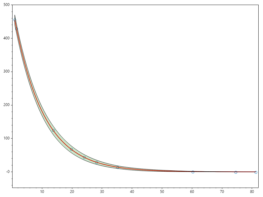

Lsqcurvefit allows the use of constraints. 1. Seed data for reproducability

Example 5C#

int seed = 23;
Random rng = new(seed);
ColVec xdata, ydata, noise = Randn(100);
double[] xstar = [2, 4, 5, 0.5];
ColVec model(ColVec x, ColVec xdata) => x[0] + x[1] * Atan(xdata - x[2]) + x[3] * xdata;
xdata = Linspace(2,7); ydata = model(xstar, xdata) + noise/10;
Scatter(xdata, ydata, "ro");
Xlabel("x"); Ylabel("y"); 
SaveAs("Seeded_Curve_Fitting_Data.png");
CloseFig();

OutputFrom the book

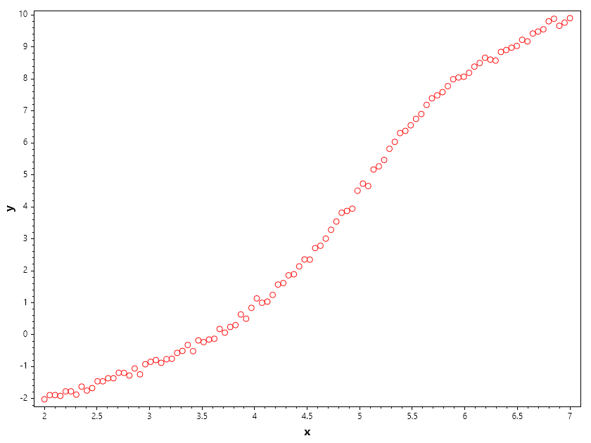
Fitting with Linear constraint

Example 6C#

int seed = 23;
Random rng = new(seed);
ColVec xdata, ydata, noise = Randn(100);
double[] xstar = [2, 4, 5, 0.5], startpt = [1, 2, 3, 1];
ColVec model(ColVec x, ColVec xdata) => x[0] + x[1] * Atan(xdata - x[2]) + x[3] * xdata;
RowVec A = new double[] { -1, -1, 1, 1 };
ColVec fineq(ColVec x) => A * x; ColVec lb = Zeros(4), ub = 7 + lb;
xdata = Linspace(2, 7); ydata = model(xstar, xdata) + noise / 10;
var opts = OptimSet(Display: true, MaxIter: 200, StepTol: 1e-6, OptimalityTol: 1e-6);
var ans = Lsqcurvefit(model, startpt, xdata, ydata, fineq, null, lb, ub, options: opts);
Console.WriteLine($"x = {ans.x.T}");
Console.WriteLine($"c = {fineq(ans.x)}");
Scatter(xdata, ydata, "ro"); HoldOn();
Plot(xdata, ans.y_hat, "-b", Linewidth: 2);
Xlabel("x"); Ylabel("y");
Legend(["Measured Data", "Model Estimate"], UpperRight);
SaveAs("Example_of_CurveFitting_using_Lsqcurvefit_with_Linear_Inequality_Constraints.png");
CloseFig();

OutputFrom the book

                                            Norm of      First-order 
 Iteration   Func-count       Resnorm          step       optimality 
     0            5          1.5768e3                       1.5131e3 
     1           11          1.2969e3     2.0985e-1         1.3141e3 
     2           17          7.9521e2     4.8334e-1         8.8913e2 
     3           23          3.0210e2     8.0528e-1         3.3710e2 
     4           29          6.1070e1     9.6797e-1         6.8593e1 
     5           35          1.0954e1     6.5846e-1         3.5873e1 
     6           41          5.9010e0     4.0095e-1         2.1176e0 
     7           47          2.8017e0     5.5907e-1         3.6019e0 
     8           53          2.0176e0     5.8269e-1         1.9446e0 
     9           59         8.8788e-1     2.3664e-1        3.6646e-1 
    10           65         7.9357e-1     4.1089e-1        4.0476e-1 
    11           71         7.8458e-1     1.5269e-1        4.7624e-2 
    12           77         7.8446e-1     1.9580e-2        1.1285e-3 
    13           83         7.8446e-1     8.1688e-4        9.1043e-6 
    14           89         7.8446e-1     1.0899e-5        3.6686e-8 
x = 
   2.2292    4.0731    4.9906    0.4498

c =   -0.8620

Example_of_CurveFitting_using_Lsqcurvefit_with_Linear_Inequality_Constraints.png

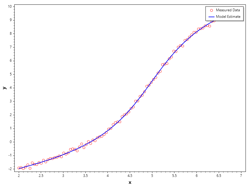
Fitting with nonlinear constraint.

Example 7C#

int seed = 23;
Random rng = new(seed);
ColVec xdata, ydata, noise = Randn(100);
double[] xstar = [2, 4, 5, 0.5], startpt = [1, 2, 3, 1];
ColVec model(ColVec x, ColVec xdata) => x[0] + x[1] * Atan(xdata - x[2]) + x[3] * xdata;
ColVec fineq(ColVec x) => x[0] * x[0] + x[1] * x[1] - 16; ColVec lb = Zeros(4), ub = 7 + lb;
xdata = Linspace(2, 7); ydata = model(xstar, xdata) + noise / 10;
var opts = OptimSet(Display: true, MaxIter: 200, StepTol: 1e-6, OptimalityTol: 1e-6);
var ans = Lsqcurvefit(model, startpt, xdata, ydata, fineq, null, lb, ub, options: opts);
Console.WriteLine($"x = {ans.x.T}");
Console.WriteLine($"c = {fineq(ans.x)}");
Scatter(xdata, ydata, "ro"); HoldOn();
Plot(xdata, ans.y_hat, "-b", Linewidth: 2);
Xlabel("x"); Ylabel("y");
Legend(["Measured Data", "Model Estimate"], UpperRight);
SaveAs("Example_of_CurveFitting_using_Lsqcurvefit_with_NonLinear_Inequality_Constraints.png");
CloseFig();

OutputFrom the book

                                            Norm of      First-order 
 Iteration   Func-count       Resnorm          step       optimality 
     0            5          1.5924e3                       1.5195e3 
     1           11          1.3067e3     2.1357e-1         1.3176e3 
     2           17          7.9492e2     4.9267e-1         8.8713e2 
     3           23          2.9268e2     8.2383e-1         3.2871e2 
     4           29          5.4477e1     9.7571e-1         7.0186e1 
     5           35          5.1316e0     6.3147e-1         3.8618e1 
     6           41          2.3496e0     2.0311e-1         4.4206e0 
     7           47          2.1077e0     1.7178e-1         1.1042e0 
     8           53          1.6958e0     3.8104e-1         1.4492e0 
     9           59          1.1900e0     6.7423e-1         1.5005e0 
    10           68          1.1570e0     6.2830e-2        6.2108e-1 
    11           76          1.1475e0     1.9324e-2        6.0844e-1 
    12           84          1.1445e0     6.0550e-3        6.0421e-1 
    13           92          1.1436e0     1.9094e-3        6.0288e-1 
    14           99          1.1429e0     1.9039e-3        6.0169e-1 
    15          105          1.1424e0     9.6744e-4        3.2159e-1 
    16          111          1.1419e0     1.0996e-3        2.4523e-1 
    17          117          1.1418e0     5.0675e-4        2.4641e-1 
    18          123          1.1418e0     7.4401e-5        2.4853e-1 
    19          129          1.1418e0     9.9412e-5        2.4946e-1 
    20          135          1.1417e0     2.9587e-4        2.5259e-1 
    21          141          1.1415e0     7.8134e-4        2.6489e-1 
    22          147          1.1414e0     2.5620e-4        2.7014e-1 
    23          153          1.1413e0     3.8591e-4        2.7899e-1 
    24          159          1.1412e0     8.9185e-4        3.0343e-1 
    25          165          1.1410e0     1.3021e-3        3.4701e-1 
    26          171          1.1410e0     8.7677e-4        3.8026e-1 
    27          177          1.1410e0     2.1676e-4        3.8888e-1 
    28          183          1.1410e0     1.7214e-5        3.8958e-1 
    29          189          1.1410e0     5.8166e-7        3.8960e-1 
x = 
   1.3361    3.7702    5.0276    0.6432

c =    0.0000

Example_of_CurveFitting_using_Lsqcurvefit_with_NonLinear_Inequality_Constraints.png