Implicit differential equations (IDEs) are a fascinating, if slightly rebellious, branch of calculus. While most standard differential equations are "explicit"—meaning you can neatly isolate the derivative on one side—IDEs keep things tangled.
Think of it like the difference between a recipe that says "Add 2 cups of flour"(explicit) and one that says "The amount of flour plus the amount of sugar must equal 5 cups" (implicit). You know the relationship, but you have to do some work to find the specific values.
What Makes an Equation Implicit?
In a standard explicit first-order ODE, we write:
dxdy=f(x,y)
In an implicit differential equation, the derivative is embedded within a function where it cannot be (or simply isn't) isolated:
F(x,y,dxdy)=0
Why Use Them?
Physics & Constraints: Many physical systems are governed by constraints (like a bead sliding on a wire) where the relationship between position and velocity is fixed by the geometry, not a direct formula.
Singularities: IDEs can describe behaviors where the derivative might become undefined or "multi-valued"(where one point has multiple possible slopes).
Differential-Algebraic Equations(DAEs): These are a subset of IDEs often used in electrical circuit simulation and multi-body dynamics.
Solving Strategies
Because you can't always "solve for y′," the approach changes:
Implicit Differentiation: If you have an equation like, x2+y2=1, you differentiate every term with respect to, treating as a function of: 2x+2ydxdy=0
Then, you isolate dxdy if possible.
Direction Fields: You can still visualize these equations! For any point, you solve the algebraic equation F(x,y,y′)=0 for y′. If there are multiple solutions for y′, the slope field might have overlapping segments.
Numerical Solvers: For complex IDEs or DAEs, standard solvers like Runge-Kutta might struggle.Specialized algorithms(like the Backward Differentiation Formula, or Diagonally implicit rungekutta) are used to handle the "stiffness" of these equations.
A Classic Example: Clairaut's Equation
One of the most famous IDEs is Clairaut's Equation: y=xdxdy+f(dxdy). This equation is unique because it often yields two types of solutions: a family of straight lines(the general solution) and a "singular solution" that acts as an envelope to those lines.
Numerical Solution
SepalSolver's Ode43i can handle implicit equations, but you need to provide the function in the form F(x,y,y′)=0. Here's a simple example of how to set up and solve an implicit equation using SepalSolver: To solve the clairaut's equation, we can rearrange it to fit the form F(x,y,y′)=0: ie , F(x,y,y′)=y−xy′−f(y′).
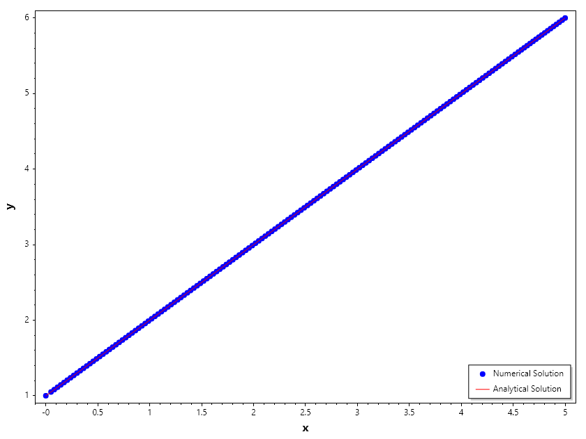
.. Admonition:: Example 1 : Solving Clairaut's Equation y=xy′+(y′)2
F(x,y,y′)=y−xy′−(y′)2,y(0)=1
First we need to compute the y′(0) from the initial condition using decic. And then we can use the computed y′(0) to solve the equation using Ode43i.
Example 1C#
1
2
3
4
5
6
7
8
9
10
11
12
13
14
15
16
17
18
19
20
21
22
23
24
25
// define the implicit function F(x, y, yp) = 0
double F(double t, double y, double yp) => y - t * yp - yp * yp;
var opts = Odeset(UserDefinedJacobian: new((t, y, yp) => 1, (t, y, yp) => -t - 2 * yp));
// initial conditions y(0) = 1, and guess for y'(0) = 0.1
double y0 = 1, yp0 = 0.1;
// Compute y'(0) using decic
(y0, yp0) = decic(F, 0, y0, 1, yp0, 0);
// Now solve the implicit ODE using Ode43i
var (T, Y, Yp) = Ode43i(F, (y0, yp0), [0, 5], opts);
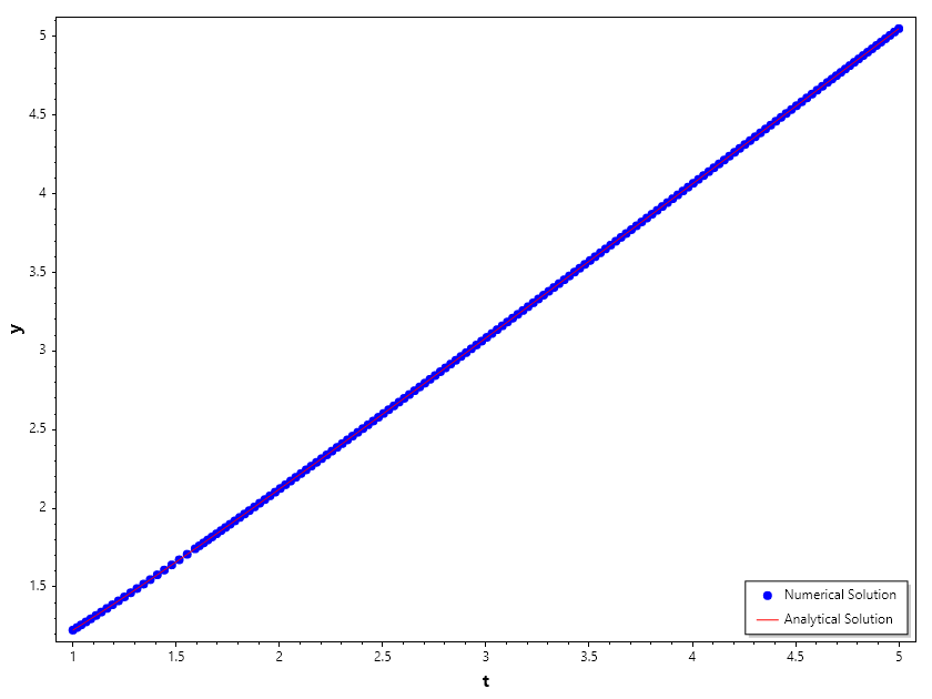
.. Admonition:: Example 2 : Solve Weissinger implicit ODE y=xnf(y′)+g(y′)
While Clairaut's equation is a textbook classic, Weissinger’s Implicit Differential Equation takes things a step further into the realm of higher-degree implicit equations. It is specifically a first-order equation where the derivative is raised to a power, but it maintains a structure that allows for a clever substitution method. The general form of a Weissinger equation is: y=xnf(y′)+g(y′)
In many contexts, particularly in the study of aerodynamics(where Weissinger’s name is prominent due to his work on lifting-line theory), you might see specialized versions of this.However, in pure mathematics, it is often treated as a generalization of d'Alembert’s equation.
1. Structure and Characteristics
Unlike a standard ODE, the Weissinger equation is nonlinear in the derivative.
Relationship to Clairaut: If you set n=1 and f(y′)=y′, you essentially return to the Clairaut form.
The Power of x: The xn term dictates how the geometry of the solution curves scales as you move away from the origin.
2. The Solution Strategy: Parameterization
To solve a Weissinger equation, we rarely try to isolate algebraically.Instead, we use a parameter, where: p=y′=dxdy substituting p into the equation gives: y=xnf(p)+g(p) To find the relationship between x and p, we differentiate the entire equation with respect to x:
dxdy=nxn−1f(p)+xnf′(p)dxdp+g′(p)dxdp
Since dxdy=p , we get a linear differential equation for in terms ofp:
p=nxn−1f(p)+[xnf′(p)+g′(p)]dxdp
This transformation is powerful because it turns a difficult implicit equation into a linear one(usually of the Bernoulli type or similar), which we can solve to get x(p). Once you have x(p) and y(fp), you have a parametric solution to the original ODE.
3. Why Weissinger Equations Matter
Weissinger's work is most famous in fluid dynamics, specifically the Weissinger Area Rule and his "L-method" for calculating lift distribution on swept wings. In these engineering contexts, implicit equations arise because the induced downwash(the change in airflow direction) depends on the lift, but the lift itself is a function of that downwash.
Applications include:
Aerodynamics: Modeling the circulation around wings with non-rectangular shapes.
Classical Mechanics: Describing trajectories where the velocity constraint is non-linear.
Singularities: Just like Clairaut equations, Weissinger equations often have "envelope" solutions where the uniqueness of the solution breaks down.
Using user defined derivative
We can also specify the derivative of the function with respect to y and y′. TO demonstrate this,
In this case, fix the initial value y(t0)=23 and let decic compute a consistent initial value for the derivative y′(t0), starting from an initial guess of y′(t0)=0.
Example 2C#
1
2
3
4
5
6
7
8
9
10
11
12
13
14
15
16
17
18
19
20
21
22
23
24
25
26
27
// Define the implicit function F(t, y, yp) = 0
double F(double t, double y, double yp) => t * y * y * yp * yp * yp - y * y * y * yp * yp + t * (t * t + 1) * yp - t * t * y;
var opts = Odeset(UserDefinedJacobian:
new((t, y, yp) => 2 * t * y * yp * yp * yp - 3 * y * y * yp * yp - t * t,
(t, y, yp) => 3 * t * y * y * yp * yp - 2 * y * y * y * yp + t * (t * t + 1)));
// Initial conditions y(t0) = sqrt(3/2), and guess for y'(t0) = 0
double t0 = 1, y0 = Sqrt(3.0 / 2.0), yp0 = 0;
// Compute y'(t0) using decic
(y0, yp0) = decic(F, t0, y0, 1, yp0, 0);
// Now solve the implicit ODE using Ode43i
var (T, Y, Yp) = Ode43i(F, (y0, yp0), [t0, 5], opts);
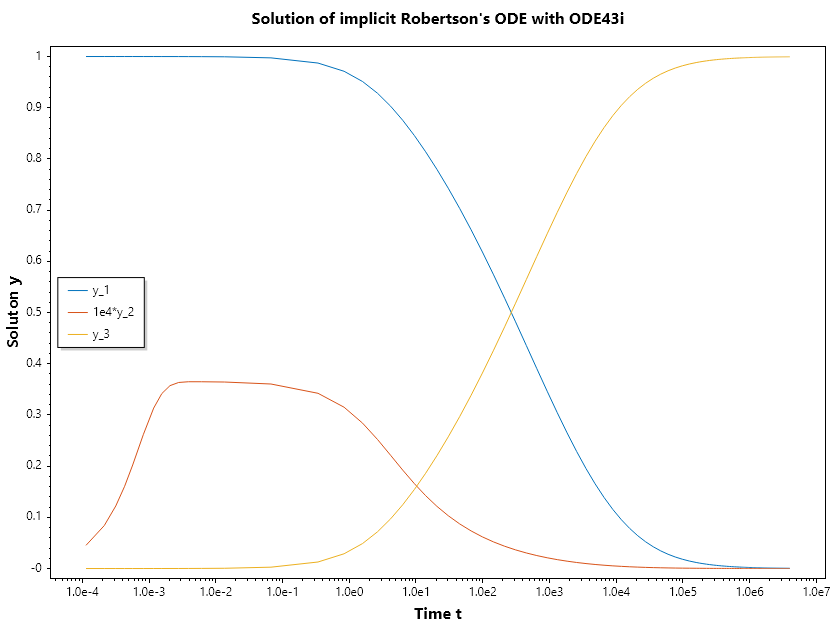
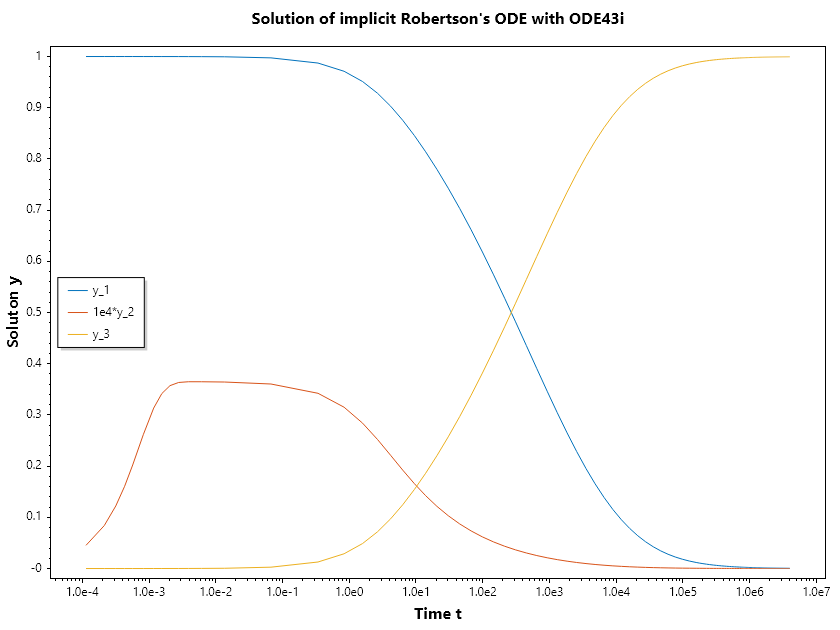
We previously solved this system of ODEs to steady state with the initial conditions y1=1, y2=0, and y3=0.
But the equations also satisfy a linear conservation law,
y1′+y2′+y3′=0
In terms of the solution and initial conditions, the conservation law is
y1+y2+y3=1.0
The problem can be rewritten as a system of DAEs by using the conservation law to determine the state of y3. This reformulates the problem as the implicit DAE system
Title("Solution of implicit Robertson's ODE with ODE43i");
SaveAs("Implicit-Robertson-ODE-Ode43i.png");
OutputFrom the book
Summary of statistics by Ode43i
        68 successful steps
        9 failed attempts
        2282 function evaluations
        77 partial derivatives
        284 LU decompositions
        1459 solutions of linear systems
Using the user defined jacobian reduces the number of function calls made during the computation.