1. Introduction to DAEs
Differential-Algebraic Equations are a class of functional equations that contain both differential equations (describing the evolution of the system) and algebraic constraints (restricting the state space). Unlike standard Ordinary Differential Equations (ODEs), DAEs are not explicitly solved for all derivatives.
A general DAE system is expressed in the implicit form:
If the Jacobian is non-singular, the system is essentially an implicit ODE. If it is singular, the system is a "true" DAE.
2. The Concept of Index
The difficulty of solving a DAE is measured by its index. The most common definition is the differentiation index: the number of times you must differentiate the algebraic constraints to express the system as a set of explicit ODEs. Index 0: An ODE. Index 1: The most common solvable DAE (e.g., the algebraic variables can be solved for directly). * Higher Index (2+): These are numerically unstable and usually require index reduction techniques before solving.
3. Solving DAEs with `sepalsolver`
In modern computational environments like C#, DAEs can be solved using the SepalSolver library, which utilizes a Mass Matrix formulation: Where is a singular matrix.
4. Examples and Applications
.. Admonition:: Example 1 :
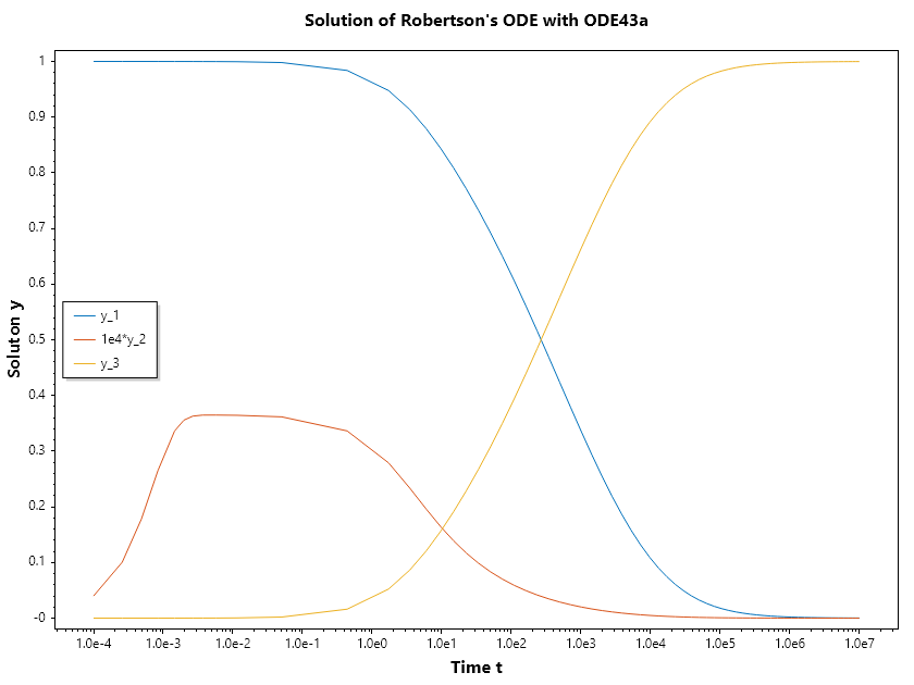
Example 1: The Robertson Problem (Chemical Kinetics) This is a classic stiff DAE representing the reaction of three species. It is an Index-1 DAE where the total mass is conserved via an algebraic constraint.
Example 1C#
.. Admonition:: Example 1 : The Simple Pendulum (Index-1)
A pendulum in Cartesian coordinates is naturally an Index-3 DAE. We solve the stabilized Index-1 version by including velocity constraints.
The position of the pendulum must satisfy the rigid rod constraint:
The Index-1 Formulation To reduce the index, we differentiate the constraint twice. The second derivative introduces the accelerations and , allowing us to solve for the Lagrange multiplier (tension).
The resulting Index-1 system is:
Example 2C#
Summary of statistics by Ode43a
        1054 successful steps
        16 failed attempts
        30517 function evaluations
        1070 partial derivatives
        4280 LU decompositions
        19799 solutions of linear systems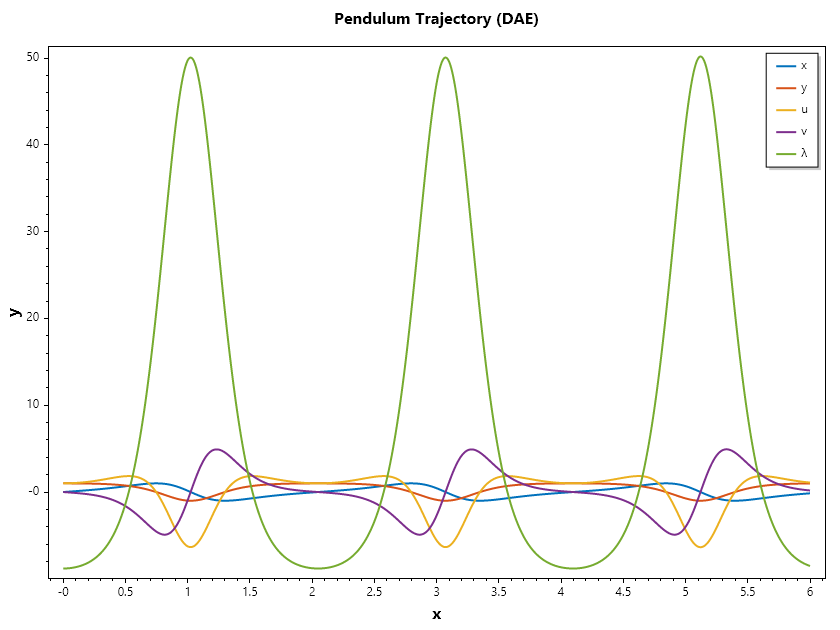
As an exercise, the reader is encouraged to solve the problem using this initial condition y0 = [1, 0, 0, 1, 1];
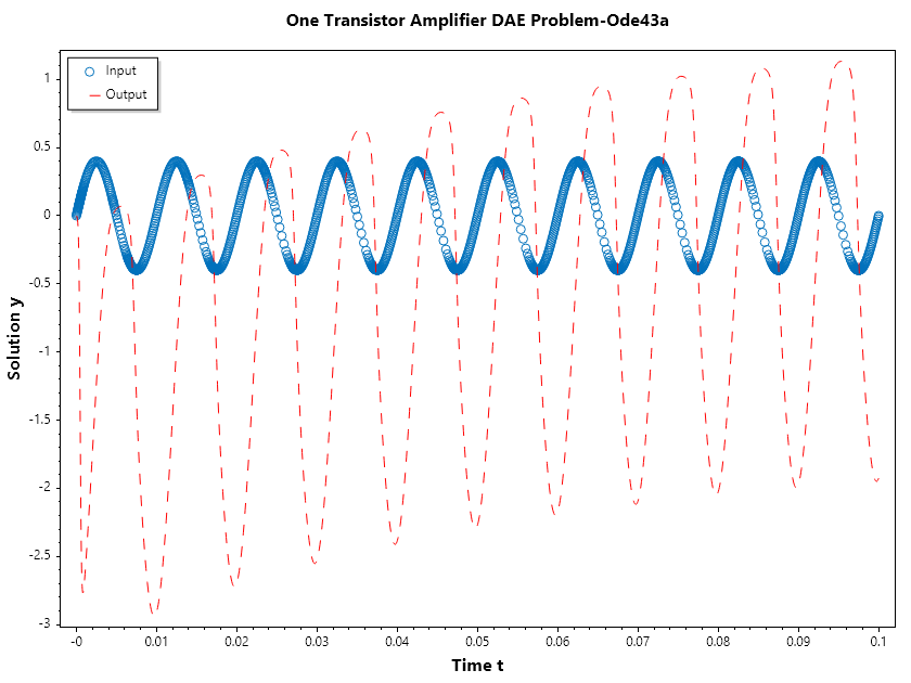
.. Admonition:: Example 2 : Semi-Explicit DAE (The Transistor Amplifier)**
This example mimics the "hbdae" problem from MathWorks, representing an electrical circuit with nonlinear components.
The transistor amplifier circuit contains six resistors, three capacitors, and a transistor.
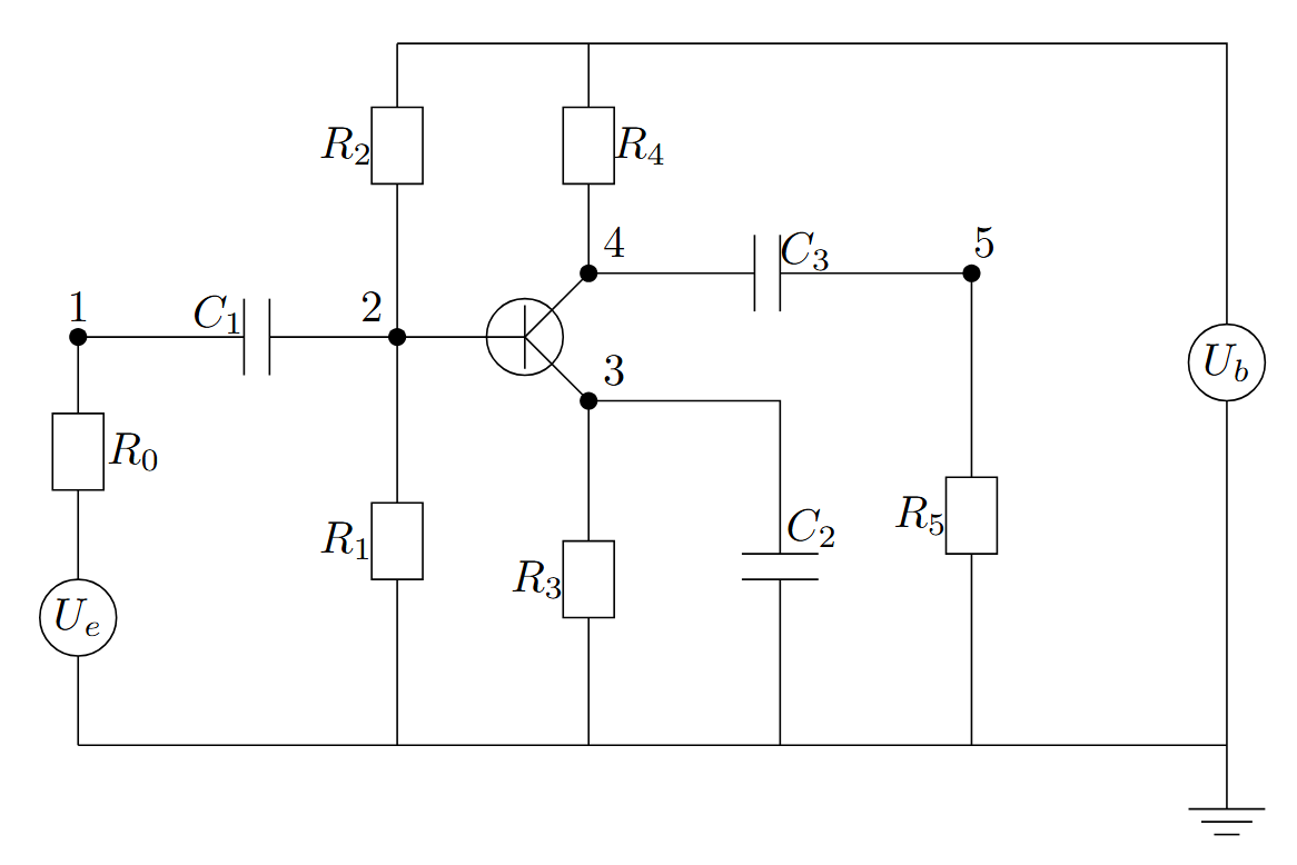
- The initial voltage signal is .
- The operating voltage is .
- The voltages at the nodes are given by: .
- The values of the resistors . are constant, and the current through each resistor satisfies .
- The values of the capacitors are constant, and the current through each capacitor satisfies .
The goal is to solve for the output voltage through node 5, . Using Kirchoff's law to equalize the current through each node (1 through 5), you can obtain a system of five equations describing the circuit:
Node 1:
Node 2:
Node 3:
Node 4:
Node 5:
By extracting the coeeficients of the derivatives into a matrix, we have:
Example 3C#
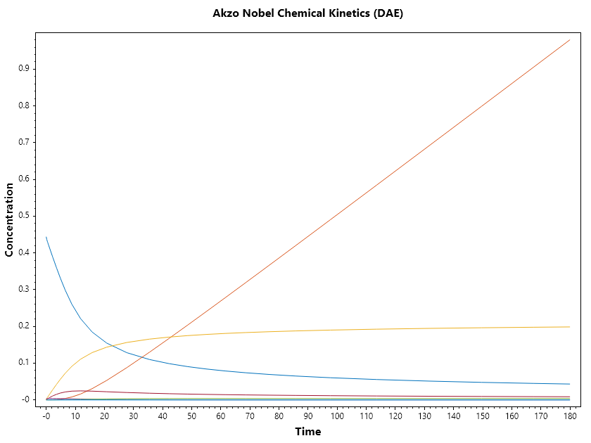
.. Admonition:: Example 3 : The Akzo Nobel Problem
A high-dimensional DAE describing a chemical process with 6 differential and 2 algebraic equations. This tests the solver's ability to handle stiff systems with coupled variables.
Mathematical Description: The system is defined by reaction rates and concentrations :
The differential equations are:
The algebraic constraints (Equilibrium):
Example 4C#
Index-2 DAE
Most DAE solvers usually avoid solving DAEs in index 2 form. But SepalSolver is able to handle most index 2 DAEs to a relative tolerance of .
Now we look at examples of index 2 DAEs
.. Admonition:: Example 4 :
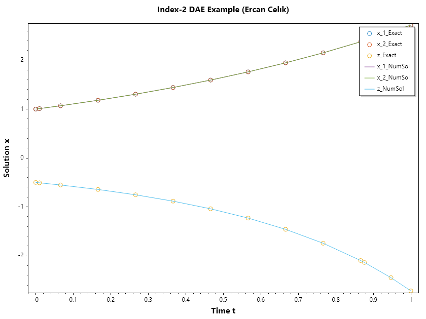
Usnig the example from "On the numerical solution of differential–algebraic equations with index-2" by Ercan Celık
Intial condition: ;
SepalSolver has the ability to compute consistent initial conditions for index 2 DAEs, so we can solve this problem without manually differentiating the algebraic constraint.
Example 5C#
Summary of statistics by Ode43a
        11 successful steps
        0 failed attempts
        486 function evaluations
        11 partial derivatives
        44 LU decompositions
        384 solutions of linear systems

    t   ||  x_1_NumSol(t)  |  x_1_Exact(t)  ||  x_2_NumSol(t)  |  x_2_Exact(t)  ||   z_NumSol(t)   |   z_Exact(t)
--------++-----------------+----------------++-----------------+----------------++-----------------+---------------
  0.00  ||     1.000000    |    1.000000    ||     1.000000    |    1.000000    ||     -0.500000   |  -0.500000
  0.01  ||     1.010050    |    1.010050    ||     1.010050    |    1.010050    ||     -0.507565   |  -0.507563
  0.11  ||     1.116229    |    1.116278    ||     1.116252    |    1.116278    ||     -0.590847   |  -0.590623
  0.21  ||     1.233620    |    1.233678    ||     1.233645    |    1.233678    ||     -0.689409   |  -0.689206
  0.31  ||     1.363366    |    1.363425    ||     1.363390    |    1.363425    ||     -0.806963   |  -0.806760
  0.41  ||     1.506760    |    1.506818    ||     1.506781    |    1.506818    ||     -0.947883   |  -0.947684
  0.51  ||     1.665236    |    1.665291    ||     1.665254    |    1.665291    ||     -1.117834   |  -1.117645
  0.61  ||     1.840381    |    1.840431    ||     1.840395    |    1.840431    ||     -1.324222   |  -1.324051
  0.71  ||     2.033947    |    2.033991    ||     2.033957    |    2.033991    ||     -1.576879   |  -1.576737
  0.81  ||     2.247872    |    2.247908    ||     2.247878    |    2.247908    ||     -1.889096   |  -1.888998
  0.91  ||     2.484298    |    2.484323    ||     2.484300    |    2.484323    ||     -2.279232   |  -2.279195
  1.00  ||     2.718273    |    2.718282    ||     2.718273    |    2.718282    ||     -2.718256   |  -2.718282


Now we compute the solution to a higher accuracy (RelTol = 1e-5):

Summary of statistics by Ode43a
        51 successful steps
        35 failed attempts
        3034 function evaluations
        86 partial derivatives
        309 LU decompositions
        2367 solutions of linear systems

    t   ||  x_1_NumSol(t)  |  x_1_Exact(t)  ||  x_2_NumSol(t)  |  x_2_Exact(t)  ||   z_NumSol(t)   |   z_Exact(t)
--------++-----------------+----------------++-----------------+----------------++-----------------+---------------
  0.00  ||     1.000000    |    1.000000    ||     1.000000    |    1.000000    ||     -0.500000   |  -0.500000
  0.01  ||     1.010050    |    1.010050    ||     1.010050    |    1.010050    ||     -0.507565   |  -0.507563
  0.05  ||     1.055859    |    1.055862    ||     1.055860    |    1.055862    ||     -0.542729   |  -0.542680
  0.10  ||     1.106491    |    1.106495    ||     1.106493    |    1.106495    ||     -0.582788   |  -0.582733
  0.15  ||     1.160230    |    1.160235    ||     1.160233    |    1.160235    ||     -0.626743   |  -0.626688
  0.20  ||     1.217541    |    1.217546    ||     1.217543    |    1.217546    ||     -0.675286   |  -0.675228
  0.25  ||     1.278831    |    1.278837    ||     1.278834    |    1.278837    ||     -0.729138   |  -0.729077
  0.30  ||     1.344534    |    1.344540    ||     1.344536    |    1.344540    ||     -0.789137   |  -0.789074
  0.35  ||     1.415157    |    1.415164    ||     1.415160    |    1.415164    ||     -0.856313   |  -0.856246
  0.40  ||     1.491307    |    1.491315    ||     1.491310    |    1.491315    ||     -0.931942   |  -0.931872
  0.45  ||     1.573719    |    1.573727    ||     1.573722    |    1.573727    ||     -1.017643   |  -1.017570
  0.51  ||     1.663297    |    1.663305    ||     1.663299    |    1.663305    ||     -1.115494   |  -1.115418
  0.57  ||     1.761180    |    1.761188    ||     1.761182    |    1.761188    ||     -1.228234   |  -1.228155
  0.63  ||     1.868846    |    1.868855    ||     1.868848    |    1.868855    ||     -1.359569   |  -1.359489
  0.69  ||     1.988277    |    1.988287    ||     1.988280    |    1.988287    ||     -1.514704   |  -1.514624
  0.69  ||     2.001288    |    2.001297    ||     2.001290    |    2.001297    ||     -1.532126   |  -1.532146
  0.75  ||     2.115598    |    2.115605    ||     2.115600    |    2.115605    ||     -1.691651   |  -1.691592
  0.76  ||     2.130305    |    2.130311    ||     2.130306    |    2.130311    ||     -1.712822   |  -1.712838
  0.76  ||     2.143131    |    2.143136    ||     2.143132    |    2.143136    ||     -1.731493   |  -1.731506
  0.77  ||     2.156035    |    2.156039    ||     2.156036    |    2.156039    ||     -1.750408   |  -1.750419
  0.77  ||     2.169016    |    2.169019    ||     2.169016    |    2.169019    ||     -1.769571   |  -1.769581
  0.78  ||     2.182075    |    2.182078    ||     2.182075    |    2.182078    ||     -1.788987   |  -1.788995
  0.79  ||     2.195212    |    2.195215    ||     2.195213    |    2.195215    ||     -1.808659   |  -1.808667
  0.79  ||     2.208429    |    2.208431    ||     2.208429    |    2.208431    ||     -1.828592   |  -1.828599
  0.80  ||     2.221725    |    2.221727    ||     2.221725    |    2.221727    ||     -1.848791   |  -1.848796
  0.80  ||     2.235101    |    2.235103    ||     2.235101    |    2.235103    ||     -1.869259   |  -1.869264
  0.81  ||     2.248557    |    2.248559    ||     2.248558    |    2.248559    ||     -1.890001   |  -1.890005
  0.82  ||     2.262095    |    2.262096    ||     2.262095    |    2.262096    ||     -1.911022   |  -1.911025
  0.82  ||     2.275714    |    2.275715    ||     2.275714    |    2.275715    ||     -1.932326   |  -1.932329
  0.83  ||     2.289415    |    2.289416    ||     2.289415    |    2.289416    ||     -1.953919   |  -1.953921
  0.83  ||     2.303198    |    2.303199    ||     2.303198    |    2.303199    ||     -1.975804   |  -1.975806
  0.84  ||     2.317065    |    2.317065    ||     2.317065    |    2.317065    ||     -1.997988   |  -1.997989
  0.85  ||     2.331014    |    2.331015    ||     2.331015    |    2.331015    ||     -2.020474   |  -2.020476
  0.85  ||     2.345048    |    2.345049    ||     2.345048    |    2.345049    ||     -2.043269   |  -2.043270
  0.86  ||     2.359167    |    2.359167    ||     2.359167    |    2.359167    ||     -2.066378   |  -2.066379
  0.86  ||     2.373370    |    2.373370    ||     2.373370    |    2.373370    ||     -2.089806   |  -2.089806
  0.87  ||     2.387659    |    2.387659    ||     2.387659    |    2.387659    ||     -2.113558   |  -2.113559
  0.88  ||     2.402033    |    2.402034    ||     2.402033    |    2.402034    ||     -2.137641   |  -2.137641
  0.88  ||     2.416495    |    2.416495    ||     2.416495    |    2.416495    ||     -2.162059   |  -2.162060
  0.89  ||     2.431043    |    2.431043    ||     2.431043    |    2.431043    ||     -2.186820   |  -2.186820
  0.89  ||     2.445679    |    2.445679    ||     2.445679    |    2.445679    ||     -2.211929   |  -2.211929
  0.90  ||     2.460403    |    2.460403    ||     2.460403    |    2.460403    ||     -2.237392   |  -2.237392
  0.91  ||     2.475216    |    2.475216    ||     2.475216    |    2.475216    ||     -2.263215   |  -2.263216
  0.91  ||     2.490118    |    2.490118    ||     2.490118    |    2.490118    ||     -2.289406   |  -2.289406
Showing the first 80 of 88 lines.
.. Admonition:: Example 5 : Pendulum position constraint (Index-2)
To reduce the index, if we differentiated the constraint once instead of twice, we end up with index 2 problem.
The resulting Index-1 system is:
Example 6C#
Summary of statistics by Ode43a
        768 successful steps
        744 failed attempts
        45119 function evaluations
        1512 partial derivatives
        4671 LU decompositions
        31359 solutions of linear systems


   0.0000   -0.0000    1.0000    1.0000    0.0000   -8.8100
   0.0600    0.0603    0.9982    1.0159   -0.0614   -8.7513
   0.1448    0.1492    0.9888    1.0920   -0.1648   -8.4683
   0.1558    0.1614    0.9869    1.1065   -0.1809   -8.4239
   0.1669    0.1737    0.9848    1.1221   -0.1979   -8.3622
   0.1780    0.1862    0.9825    1.1387   -0.2158   -8.2949
   0.1890    0.1989    0.9800    1.1563   -0.2347   -8.2215
   0.2001    0.2118    0.9773    1.1749   -0.2546   -8.1419
   0.2112    0.2249    0.9744    1.1945   -0.2757   -8.0555
   0.2222    0.2383    0.9712    1.2150   -0.2981   -7.9621
   0.2333    0.2518    0.9678    1.2364   -0.3217   -7.8612
   0.2444    0.2656    0.9641    1.2588   -0.3468   -7.7523
   0.2554    0.2797    0.9601    1.2820   -0.3735   -7.6350
   0.2665    0.2940    0.9558    1.3060   -0.4017   -7.5088
   0.2776    0.3086    0.9512    1.3309   -0.4318   -7.3731
   0.2886    0.3235    0.9462    1.3564   -0.4637   -7.2273
   0.2997    0.3386    0.9409    1.3826   -0.4976   -7.0708
   0.3108    0.3541    0.9352    1.4094   -0.5336   -6.9029
   0.3218    0.3698    0.9291    1.4367   -0.5718   -6.7229
   0.3329    0.3859    0.9226    1.4644   -0.6125   -6.5301
   0.3440    0.4022    0.9155    1.4924   -0.6557   -6.3236
   0.3550    0.4189    0.9080    1.5206   -0.7015   -6.1026
   0.3661    0.4359    0.9000    1.5489   -0.7502   -5.8662
   0.3772    0.4532    0.8914    1.5772   -0.8018   -5.6135
   0.3882    0.4708    0.8822    1.6052   -0.8566   -5.3435
   0.3993    0.4887    0.8725    1.6328   -0.9147   -5.0551
   0.4104    0.5069    0.8620    1.6598   -0.9761   -4.7472
   0.4214    0.5255    0.8508    1.6860   -1.0412   -4.4187
   0.4325    0.5443    0.8389    1.7111   -1.1101   -4.0684
   0.4436    0.5633    0.8262    1.7350   -1.1829   -3.6951
   0.4546    0.5826    0.8127    1.7571   -1.2597   -3.2973
   0.4657    0.6022    0.7983    1.7774   -1.3407   -2.8739
   0.4766    0.6216    0.7833    1.7951   -1.4246   -2.4314
   0.4872    0.6408    0.7677    1.8098   -1.5105   -1.9732
   0.4976    0.6596    0.7516    1.8215   -1.5985   -1.4990
   0.5077    0.6781    0.7350    1.8301   -1.6885   -1.0086
   0.5176    0.6963    0.7177    1.8352   -1.7805   -0.5015
   0.5274    0.7142    0.6999    1.8369   -1.8744    0.0225
   0.5370    0.7318    0.6815    1.8349   -1.9702    0.5640
   0.5463    0.7489    0.6627    1.8291   -2.0671    1.1190
   0.5554    0.7656    0.6434    1.8194   -2.1650    1.6872
   0.5644    0.7817    0.6236    1.8058   -2.2637    2.2684
   0.5731    0.7974    0.6034    1.7881   -2.3631    2.8630
   0.5816    0.8127    0.5827    1.7663   -2.4631    3.4711
   0.5901    0.8274    0.5616    1.7402   -2.5637    4.0925
   0.5983    0.8416    0.5401    1.7099   -2.6647    4.7276
   0.6064    0.8554    0.5180    1.6751   -2.7660    5.3761
   0.6144    0.8686    0.4955    1.6358   -2.8675    6.0382
   0.6223    0.8813    0.4726    1.5919   -2.9689    6.7139
   0.6300    0.8935    0.4491    1.5434   -3.0702    7.4030
   0.6377    0.9051    0.4253    1.4900   -3.1712    8.1055
   0.6452    0.9161    0.4009    1.4318   -3.2716    8.8214
   0.6527    0.9266    0.3762    1.3687   -3.3714    9.5505
   0.6601    0.9364    0.3509    1.3006   -3.4703   10.2928
   0.6674    0.9456    0.3253    1.2274   -3.5682   11.0481
   0.6746    0.9542    0.2992    1.1490   -3.6647   11.8163
   0.6817    0.9621    0.2726    1.0654   -3.7598   12.5971
   0.6888    0.9694    0.2457    0.9765   -3.8531   13.3906
   0.6958    0.9759    0.2183    0.8823   -3.9444   14.1963
   0.7028    0.9817    0.1905    0.7827   -4.0336   15.0142
   0.7097    0.9867    0.1623    0.6777   -4.1202   15.8441
   0.7166    0.9910    0.1337    0.5672   -4.2042   16.6856
   0.7232    0.9944    0.1059    0.4558   -4.2820   17.5053
   0.7290    0.9968    0.0805    0.3513   -4.3494   18.2509
   0.7342    0.9983    0.0576    0.2544   -4.4074   18.9242
   0.7389    0.9993    0.0372    0.1657   -4.4569   19.5267
   0.7429    0.9998    0.0191    0.0861   -4.4986   20.0568
   0.7463    1.0000    0.0038    0.0172   -4.5327   20.5086
Showing the first 80 of 781 lines.
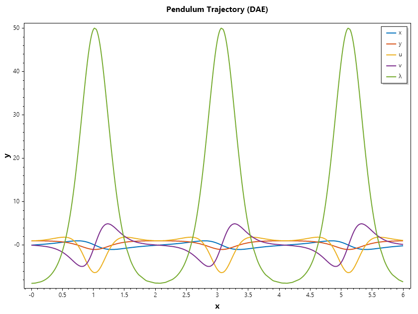
Observe that the initial condition supplied for was ; but the result returned shown that the correct initial condition for the algebraic variable is . Sending in a wrong initial condition was done on purpose, to test the ability of sepalsolver to compute the initial condition of the algebraic variable.
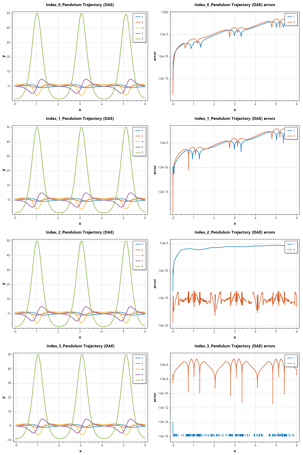
<header> Solving Index 3 </header> To show more capability of the sepalsolver with higher index DAEs, we present this solution of the Pendulum equation from index 0 to index 3 below
% --- Index 0 ---
% --- Index 1 ---
% --- Index 2 ---
% --- Index 3 ---
The result is assessed using these errors
Example 7C#
Summary of statistics by Ode45
        192 successful steps
        3 failed attempts
        1171 function evaluations

Summary of statistics by Ode43a
        1054 successful steps
        16 failed attempts
        30517 function evaluations
        1070 partial derivatives
        4280 LU decompositions
        19799 solutions of linear systems

Summary of statistics by Ode43a
        831 successful steps
        15 failed attempts
        31650 function evaluations
        846 partial derivatives
        3384 LU decompositions
        23173 solutions of linear systems

Summary of statistics by Ode43a
        8756 successful steps
        19 failed attempts
        282381 function evaluations
        8775 partial derivatives
        35097 LU decompositions
        194608 solutions of linear systems