Reineur Solver: solve real-world problems with confidence

Stiff Differential Equations

In the world of numerical simulation, Stiffness is a phenomenon where certain terms in a differential equation lead to extremely rapid changes in the solution, even if the overall behavior of the system is smooth. It is not a mathematical property of the equation itself, but rather a practical limitation of the numerical methods used to solve it.A system is generally considered "stiff" when there is a large disparity between the fastest and slowest "time scales" in the problem.

The "Stability Trap" Standard explicit solvers (like the classic Runge-Kutta 4th Order) work by taking small steps based on the current slope. In a stiff system, if the step size $\Delta t$ is even slightly too large, the solver will "overcorrect" for a rapid transient, leading to wild oscillations and eventually a total crash (divergence).To maintain stability in a stiff system, an explicit solver is forced to take steps so infinitesimally small that the simulation may take days or years to complete, even though the physical system being modeled is barely changing.

Engineering Usage Examples

Stiff equations appear whenever a system involves processes that happen at vastly different speeds simultaneously.

1. Chemical Kinetics and Combustion

In a car engine's combustion chamber, some chemical reactions occur in microseconds (the creation of free radicals), while the overall combustion process and the movement of the piston take milliseconds. To model the exhaust emissions accurately, you must solve a stiff system that captures both the "lightning-fast" chemistry and the "slow" mechanical motion.

2. Electronic Circuit Simulation

In high-frequency power electronics, a circuit might have a capacitor that charges in nanoseconds alongside a cooling system that responds over minutes. Standard simulators would choke on the nanosecond transients; stiff solvers allow the simulation to "step over" the fast transients once they have stabilized.

3. Stiffness in Structural Mechanics

A stiffly-supported beam or a very rigid spring system (high spring constant $k$) creates equations where high-frequency vibrations exist alongside slow, large-scale deflections. Stiff solvers are required to ensure the high-frequency "noise" doesn't blow up the math of the "signal."

Solving Strategy: Implicit Methods

The cure for stiffness is the use of Implicit Methods (such as Backward Euler or BDF - Backward Differentiation Formulas and Diagonally Implicit Runge Kuttas).Unlike explicit methods that look at where the system is, implicit methods look at where the system is going by solving an algebraic equation at every step. While this requires more CPU power per step (often involving a matrix inversion), it allows for much larger time steps without losing stability.

Examples

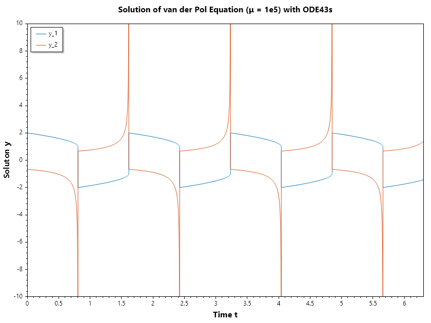
SepalSolver impelements ODE43s for stiff differential equation. This is an embeded diagonally implicit solver which is capable of error estimate and hence enable adpative time stepping. Here we look at how to use this function to solve stiff Van der Pol Oscillator and Robertson differential equation.

.. Admonition:: Example 1 : Van der Pol Oscillator ( $\mu = 1 \times 10^5$ )

Solve the ODE $~d^2y/dt^2 = 10^{5}((1 - y^2)y' - y)~$ with initial condition $~y(0) = [2, 0]~$ over the interval $[0, 6.3]$ .

First we have to convert this to a system of first order differential equations,

\begin{array}{rcl} y' &=& v \\ v' &=& 10^{5}((1 - y^2)v - y) \end{array}

Example 1C#

//define ODE
double[] vdp2(double t, double[] y)=>
    [y[1], 1e5*((1 - y[0] * y[0]) * y[1] - y[0])];
//Solve ODE
(ColVec T, Matrix Y) = Ode43s(vdp2, [2, 0], [0, 6.3]);
// Plot the result
Plot(T, Y);
Axis([0, 6.3, -10, 10]);
Xlabel("Time t"); Ylabel("Soluton y");
Legend(["y_1", "y_2"], UpperLeft);
Title("Solution of van der Pol Equation (μ = 1e5) with ODE43s");
SaveAs("Van-der-Pol-μ=1e5-Ode43s.png");

OutputFrom the book

.. Admonition:: Example 2 : Robertson ODE

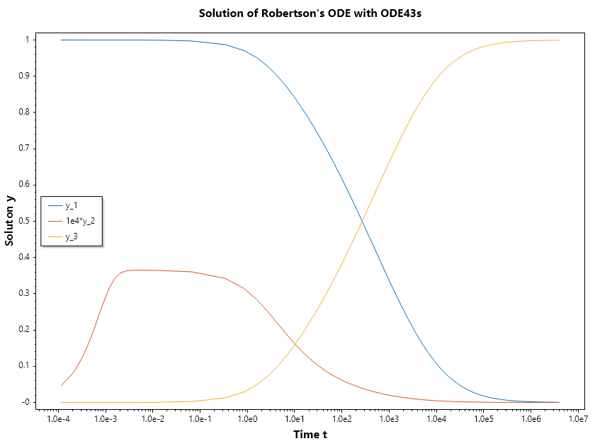
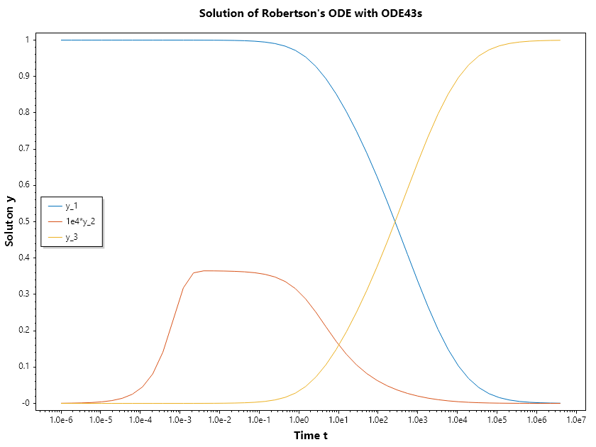
The Robertson ODE is the classic "benchmark" problem used to test the efficiency and stability of numerical solvers for stiff differential equations. It describes a simplified chemical reaction involving three species ( $y_1, y_2, y_3$ ) with reaction rates that differ by several orders of magnitude.

The Reaction Network The system models the following three reactions:

$y_1 \xrightarrow{0.04} y_2$ (Slow)

$y_2 + y_2 \xrightarrow{3 \cdot 10^7} y_3 + y_2$ (Very Fast)

$y_2 + y_3 \xrightarrow{10^4} y_1 + y_3$ (Fast)

The resulting system of differential equations is:

$\cfrac{dy_1}{dt} = -0.04y_1 + 10^4 y_2 y_3$

$\cfrac{dy_2}{dt} = 0.04y_1 - 10^4 y_2 y_3 -3 \cdot 10^7 y_2^2$

$\cfrac{dy_3}{dt} = 3 \cdot 10^7 y_2^2$

Example 2C#

//define ODE
double[] robertson(double t, double[] y) =>
    [-0.04 * y[0] + 1e4 * y[1]*y[2],
      0.04 * y[0] - 1e4 * y[1]*y[2] - 3e7*y[1]*y[1],
      3e7*y[1]*y[1]];
//Solve ODE
(ColVec T, Matrix Y) = Ode43s(robertson, [1, 0, 0], [0, 4e6]);
// Plot the result
Y[.., 1] = 1e4*Y[.., 1];
SemiLogx(T, Y);
Xlabel("Time t"); Ylabel("Soluton y");
Legend(["y_1", "1e4*y_2", "y_3"], MiddleLeft);
Title("Solution of Robertson's ODE with ODE43s");
SaveAs("Robertson-ODE-Ode43s.png");

OutputFrom the book

Example 3C#

//define ODE
double[] robertson(double t, double[] y) =>
    [-0.04 * y[0] + 1e4 * y[1]*y[2],
      0.04 * y[0] - 1e4 * y[1]*y[2] - 3e7*y[1]*y[1],
      3e7*y[1]*y[1]];
//Solve ODE
//Now we want the results to be computed at
//logarithmically evenly spaced points from 1e-6 to 4e6
(ColVec T, Matrix Y) = Ode43s(robertson, [1, 0, 0], [0, ..Logspace(-6, 6.6)]);
// Plot the result
Y[.., 1] = 1e4*Y[.., 1];
SemiLogx(T, Y);
Xlabel("Time t"); Ylabel("Soluton y");
Legend(["y_1", "1e4*y_2", "y_3"], MiddleLeft);
Title("Solution of Robertson's ODE with ODE43s");
SaveAs("Robertson-ODE-given-points-Ode43s.png");

OutputFrom the book

.. Admonition:: Example 4 : Using OdeSet

Here we look at the use of odeset

Example 4C#

//define ODE
double[] robertson(double t, double[] y) =>
    [-0.04 * y[0] + 1e4 * y[1]*y[2],
      0.04 * y[0] - 1e4 * y[1]*y[2] - 3e7*y[1]*y[1],
      3e7*y[1]*y[1]];
//Solve ODE
// Here we chose reltol = 1e-4(defult is 1e-3), abstol = 1e-7(default is 1e-6)
var opts = Odeset(RelTol: 1e-4, AbsTol: 1e-7);
(ColVec T, Matrix Y) = Ode43s(robertson, [1, 0, 0], [0, .. Logspace(-6, 6.6)], opts);

Example 5C#

//define ODE
double[] robertson(double t, double[] y) =>
    [-0.04 * y[0] + 1e4 * y[1]*y[2],
      0.04 * y[0] - 1e4 * y[1]*y[2] - 3e7*y[1]*y[1],
      3e7*y[1]*y[1]];
//Solve ODE
var opts = Odeset(Stats: true);
Console.WriteLine("Computational Cost Using Default Tolerance Setting:");
Ode43s(robertson, [1, 0, 0], [0, .. Logspace(-6, 6.6)], opts);
Console.WriteLine("\n\n");
opts = Odeset(Stats: true, RelTol: 1e-4, AbsTol: 1e-7);
Console.WriteLine("Computational Cost Using Custom Tolerance Setting");
Ode43s(robertson, [1, 0, 0], [0, .. Logspace(-6, 6.6)], opts);

OutputFrom the book

Computational Cost Using Default Tolerance Setting:
Summary of statistics by Ode43s
        119 successful steps
        0 failed attempts
        2888 function evaluations
        119 partial derivatives
        476 LU decompositions
        1935 solutions of linear systems




Computational Cost Using Custom Tolerance Setting
Summary of statistics by Ode43s
        180 successful steps
        0 failed attempts
        4711 function evaluations
        180 partial derivatives
        720 LU decompositions
        3270 solutions of linear systems

Takes a free account.

Stiff Differntial Equations

Stiff Differential Equations

Engineering Usage Examples

1. Chemical Kinetics and Combustion

2. Electronic Circuit Simulation

3. Stiffness in Structural Mechanics

Solving Strategy: Implicit Methods

Examples