NonLinear System — SepalSolver

The SepalSolver function Fsolve is used to solve systems of nonlinear equations. It finds a vector $\mathbf{x}$ such that:

\mathbf{f}(\mathbf{x}) = \mathbf{0}

Unlike Fzero, which works for single-variable equations, Fsolve is designed for multivariable problems.

Syntax

The basic syntax is:

Example 1C#

x = Fsolve(fun, x0);

Where:

fun : Function handle that returns a vector of equations.
x0 : Initial guess for the solution vector.

Just like the case of Fzero, we can use SolverSet to configure the solver and gain a window into what is going on under the hood.

Example 2C#

var options = SolverSet(Display: true);
x = fsolve(fun, x0, options);

How fsolve Works

fsolve uses iterative numerical methods such as:
Newton Raphson Algorithm (default, robust for many problems).
Forward Differencing for Numerical differentiation of the function
**LU rank 1 update to directly update the LU factors reducing the neet for repeated factorization.
It requires a good initial guess because nonlinear systems may have multiple solutions or none at all.

Examples

.. Admonition:: Example 1 : : Single Equation

Solve: $x^2 - 4 = 0$ :

Example 3C#

double fun(double x) => x*Sin(x) - 0.5;
double x0 = 1;
double root = Fsolve(fun, x0);
Console.WriteLine($"root = {root}");

OutputFrom the book

root = 0.7408409563514429

.. Admonition:: Example 2 : System of Equations

Solve the system:

\begin{array}{c} 3x_1 - \cos(x_2 x_3) - \cfrac{1}{2} = 0 \\ x_1^2 - 81(x_2+0.1)^2 + \sin(x_3) + 1.06 = 0 \\ e^{x_1x_2} +20x_3 + \cfrac{10\pi-3}{3} = 0 \end{array}

Where: $x_0 = [0.1, 0.1, -0.1]^T$

Example 4C#

double[] fun(double[] x) => [3 * x[0] - Cos(x[1] * x[2]) - 0.5,
                             x[0] * x[0] - 81*Pow(x[1] + 0.1, 2) + Sin(x[2]) + 1.06,
                             Exp(-x[0] * x[1]) + 20 * x[2] + (10 * pi - 3) / 3];
// set initial guess
double[] x0 = [0.1, 0.1, -0.1];
// call the solver
var x = Fsolve(fun, x0);
// display the result
Console.WriteLine(x);

OutputFrom the book

 0.5000
 0.0000
-0.5236

Just like the case of single variable nonlinear equation, nonlinear system can also be solved using automatic differentiation class

Example 5C#

AutoDiff[] fun(AutoDiff[] x) => [3 * x[0] - Cos(x[1] * x[2]) - 0.5,
                     x[0] * x[0] - 81*Pow(x[1] + 0.1, 2) + Sin(x[2]) + 1.06,
                     Exp(-x[0] * x[1]) + 20 * x[2] + (10 * pi - 3) / 3];
// set initial guess
double[] x0 = [0.1, 0.1, -0.1];
// call the solver
var opts = SolverSet(Display: true);
var x = Fsolve(fun, x0, opts);
// display the result
Console.WriteLine(x);

OutputFrom the book

Iteration    Func-count       f(x)      Norm of Step
    0            1             0           Start
    1            2          0.34586       0.58656     
    2            3          0.02588       0.01799     
    3            4        2.012e-004      0.00157     
    4            5        1.254e-008     1.245e-005   
    5            6        1.776e-015     7.761e-010   

  0.5000
  0.0000
 -0.5236

Applications

Engineering: Nonlinear circuit analysis, chemical equilibrium.
Physics: Solving coupled nonlinear equations in dynamics.
Optimization: Finding stationary points of nonlinear functions.

Limitations

Requires a good initial guess; poor guesses may lead to divergence.
May converge to local solutions rather than global ones.
Sensitive to scaling of equations.

Comparison with fzero

Feature	`fzero`	`fsolve`
Problem type	Single nonlinear equation	System of nonlinear equations
Input	Function handle, scalar or interval	Function handle, vector initial guess
Methods used	Bisection, secant, inverse quadratic interp	Newton-Raphson's method
Output	Scalar root	Vector solution

Parameterized Equations

Parameterized nonlinear equations $F(x, \lambda) = 0$ are equations or systems of equations that depend on one or more parameters: $\lambda$ . They are widely used in mathematics, engineering, and economics to study how solutions change as parameters vary, enabling sensitivity analysis, bifurcation studies, and optimization.

This parameter(s) can be exploited to provide means to guarantee that a good initial guess can be estimated. For instance, some values of the parameter might help eliminate the nonlinearity of the system and hence, no guess is needed for the solution. Then variation of this parameter can then be used to move the solution $x$ gently to their values that corresponds to the orginally intended values of the parameter $\lambda$ .

.. Admonition:: Example 2 :

Consider this parameterized nonlinear system. The nonlinearity is controlled by parameter $c$ .

\begin{array}{c} 2x + y - \exp(-cx) = 0 \\ -x + 2y - \exp(-cy) = 0 \end{array}

Setting $c = 0$ , turns this system into a linear system with solution of $[x,y] = [0.2, 0.6]$ Hence, we can gradually change $c$ from $0$ to $20$ , while solving for $[x, y]$ .

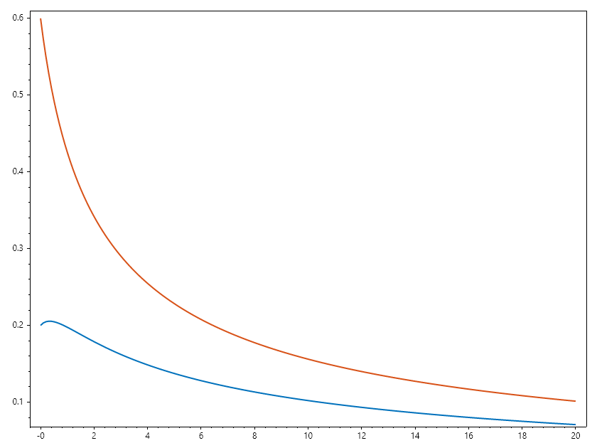
Example 6C#

// Parameterized nonlinear equations
double[] paramfun(ColVec x, double c)
{
    return [ 2*x[0] + x[1]  - Exp(-c*x[0]),
    -x[0] + 2*x[1]  - Exp(-c*x[1])];
}
// variatiob of c from 0 to 20.
RowVec C = Linspace(0, 20, 200);
// initial guess as solution of linear system when c = 0.
ColVec x = new double[] { 0.2, 0.6 };
// setting maximum iteration number
var opts = SolverSet(MaxIter: 1000);
Matrix X = C.Select(c => x = Fsolve(x => paramfun(x, c), x, opts)).ToList();
Plot(C, X, Linewidth: 2);
SaveAs("Parameterozed_Nonlinear_Equations.png");

OutputFrom the book

Matrix Equation

The SepalSolver also allow for easy computation of matrix equations. For instance, we can easily compute the cuberoot of a matrix. $x^3 = \begin{pmatrix} 1&2 \\ 3&4 \end{pmatrix}$ ;

.. Admonition:: Example 3 :

x^3 = \begin{pmatrix} 1&2 \\ 3&4 \end{pmatrix}

Example 7C#

// Solve Nonlinear System of Polynomials
Matrix A = new double[,]
{
    {1, 2},
    {3, 4}
};
var opts = SolverSet(Display: true);
Matrix x = Fsolve(x => x*x*x - A, Ones(2, 2), opts);
Console.WriteLine(x);

OutputFrom the book

Iteration    Func-count       f(x)      Norm of Step
    0            1          3.74165        start      
    1            6          0.94293       0.61237     
    2            7          2661960       6432.80     
    3            8          0.45614       6432.80     
    4            9          0.39097       0.05487     
    5            10         0.39548       0.03847     
    6            11         0.39690       0.00219     
    7            12         0.39702      1.712e-004   
    8            17         263.674       6.34236     
    9            18         0.37461       6.33363     
    10           19         0.37411       0.00901     
    11           20         3.91142       1.47633     
    12           21         0.35406       1.34995     
    13           22         0.31481       0.11135     
    14           23         1.75353       0.89775     
    15           24         0.22618       0.76114     
    16           29         0.13103       0.26771     
    17           30         0.03317       0.09820     
    18           31         0.00338       0.01983     
    19           32       1.047e-004      0.00225     
    20           33       3.140e-007     6.762e-005   
    21           34       2.926e-011     2.022e-007   

 -0.1291    0.8602
  1.2903    1.1612

Summary

Fsolve is SelapSolver’s go-to tool for solving nonlinear systems. It is powerful and flexible, but demands careful choice of initial guesses and problem formulation to ensure convergence.