Nonlinear Equation — SepalSolver

Root of a nonlinear equation near initial guess $x_0$ can be found using Fzero or Fsolve. It numerically locates a value: $x$ such that: $f(x) = 0$ . This is particularly useful when analytical solutions are difficult or impossible to obtain.

To solve the equation: $x\exp(x) = 2$ , start with initial guess of $x_0 = 0.5$ ;

Example 1C#

//Single nonlinear equation
double f(double x) => x * Exp(x) - 2;
// solve equation using fzero
double x = Fzero(f, 0.5);
Console.WriteLine($"x = {x}");

OutputFrom the book

x = 0.8526055020137255

In this case, Fzero first search for an interval that brackets the root. Then uses brent's method to hone in on the root. If we are sure of the interval containing the root, we can save the effort spent on bracketing the root by supplying that.

Example 2C#

//Single nonlinear equation (bracketted)
double f(double x) => x * Exp(x) - 2;
double x = Fzero(f, [0.5, 1]);
Console.WriteLine($"x = {x}");

OutputFrom the book

x = 0.8526055020137254

To have window into the solution process, we can using solver setting SolverSet() to get the solver to print out the result after each iteration.

Example 3C#

// Single nonlinear equation
double f(double x) => x * Exp(x) - 2;
// set solver behaviour
var opts = SolverSet(Display: true);
// solve equation using fzero
double x = Fzero(f, 0.5, opts);
Console.WriteLine($"x = {x}");

OutputFrom the book

 Search for an interval around 0.5 containing a sign change:
fun-count     a          f(a)           b          f(b)     Procedure 
    1         5e-1   -1.1756e+0         5e-1   -1.1756e+0   initial interval 
    3    4.7172e-1    -1.244e+0    5.2828e-1    -1.104e+0   search          
    5       4.6e-1   -1.2713e+0       5.4e-1   -1.0734e+0   search          
    7    4.4343e-1   -1.3091e+0    5.5657e-1    -1.029e+0   search          
    9       4.2e-1   -1.3608e+0       5.8e-1    -9.641e-1   search          
   11    3.8686e-1   -1.4304e+0    6.1314e-1   -8.6802e-1   search          
   13       3.4e-1   -1.5223e+0       6.6e-1   -7.2304e-1   search          
   15    2.7373e-1   -1.6401e+0    7.2627e-1   -4.9853e-1   search          
   17       1.8e-1   -1.7845e+0       8.2e-1   -1.3819e-1   search          
   19    4.7452e-2   -1.9502e+0    9.5255e-1     4.693e-1   search          

 Solving for solution between 0.047452 and 0.952548
fun-count     x         f(x)       Procedure 
   19    9.5255e-1     4.693e-1    initial        
   20    7.7699e-1    -3.101e-1    interpolation  
   21    8.4684e-1   -2.4938e-2    interpolation  
   22    8.5264e-1    1.5721e-4    interpolation  
   23    8.5261e-1   -6.9891e-7    interpolation  
   24    8.5261e-1  -1.9465e-11    interpolation  
   25    8.5261e-1         0e+0    interpolation  
x = 0.8526055020137255

by setting the solver setting in the case of bracketed root, we can see how the solution process differs from the case of a single initial guess.

Example 4C#

// Single nonlinear equation
double f(double x) => x * Exp(x) - 2;
// set solver behaviour
var opts = SolverSet(Display: true);
// solve equation using fzero
double x = Fzero(f, [0.5, 1], opts);
Console.WriteLine($"x = {x}");

OutputFrom the book

fun-count     x         f(x)       Procedure 
    2         1e+0    7.1828e-1    initial        
    3    8.1037e-1   -1.7768e-1    interpolation  
    4    8.4798e-1    -2.004e-2    interpolation  
    5    8.5263e-1    9.9913e-5    interpolation  
    6    8.5261e-1   -3.5651e-7    interpolation  
    7    8.5261e-1  -6.3105e-12    interpolation  
    8    8.5261e-1  -2.2204e-16    interpolation  
x = 0.8526055020137254

SepalSolver also has gradient based "Fsolve", which can use finite difference, user defined functions, or automatic differentiation methods to evaluate the gradient. How to do this is demonstrated in the following example.

Using finite difference

Example 5C#

// define the function
double fun(double x) => 3 * x - Cos(x * x) - 0.5;
// set initial guess
double x0 = 0.1;
// call the solver
var opts = SolverSet(Display: true);
var x = Fsolve(fun, x0, opts);
// display the result
Console.WriteLine($"x = {x}");

OutputFrom the book

Func-count      x               f(x) 
     1      1.00000E-1     -1.19995E+0
     4      4.99717E-1      3.01682E-2
     7      4.90426E-1      6.23684E-5
    10      4.90406E-1     2.62400E-10
x = 0.4904064540069147

Using user defined function example

Example 6C#

// define the function
double fun(double x) => 3 * x - Cos(x * x) - 0.5;
// set initial guess
double x0 = 0.1;
// call the solver
Func<double, double> userJacobian = x => 3 + 2 * x * Sin(x * x);
var opts = SolverSet(Display: true, UserDefinedJac: userJacobian);
var x = Fsolve(fun, x0, opts);
// display the result
Console.WriteLine($"x = {x}");

OutputFrom the book

Func-count      x               f(x) 
     1      1.00000E-1     -1.19995E+0
     2      4.99717E-1      3.01682E-2
     3      4.90426E-1      6.23684E-5
     4      4.90406E-1     2.62401E-10
x = 0.49040645400691485

Using automatic differentiation example

Example 7C#

// define the function (the variable must be of the type AUTODIFF)
AutoDiff fun(AutoDiff x) => 3 * x - Cos(x * x) - 0.5;
// set initial guess
double x0 = 0.1;
// call the solver
var opts = SolverSet(Display: true);
var x = Fsolve(fun, x0, opts);
// display the result
Console.WriteLine($"x = {x}");

OutputFrom the book

Func-count      x               f(x) 
     1      1.00000E-1     -1.19995E+0
     2      4.99717E-1      3.01682E-2
     3      4.90426E-1      6.23684E-5
     4      4.90406E-1     2.62401E-10
x = 0.49040645400691485

Practical Application

The gas compressibility factor (Z-factor) measures how much a real gas deviates from ideal gas behavior. It is defined as:

Z = \frac{P V}{n R T}

where:

$P$ = pressure
$V$ = volume
$n$ = number of moles
$R$ = gas constant
$T$ = temperature

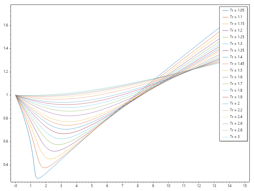
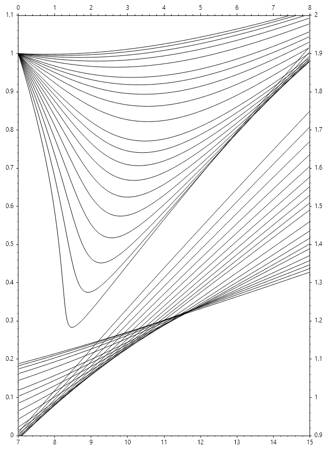
Accurate determination of $Z$ is essential in petroleum engineering for reservoir simulation, material balance, and pipeline design. Unlike explicit correlations, which provide $Z$ directly as a function of pseudo-reduced pressure ( $P_{pr}$ ) and pseudo-reduced temperature ( $T_{pr}$ ), implicit correlations require solving an equation iteratively because $Z$ appears on both sides of the equation.

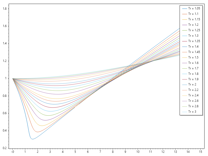
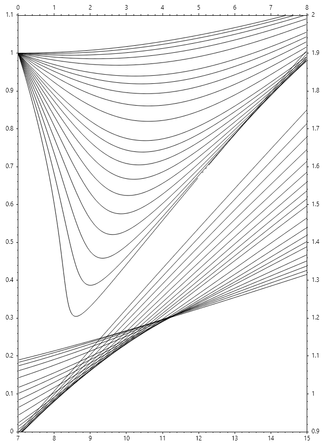
The Hall–Yarbrough correlation (1973) is one of the most widely used implicit methods for estimating Z. It was developed based on the hard-sphere equation of state and tested against multiple reservoir gas systems. The general form is:

\begin{array}{c} A = 0.06125t \exp\left(-1.2(1 - t)^2\right) \\ B = 14.76t - 9.76t^2 + 4.58t^3 \\ C = 90.7t - 242.2t^2 + 42.4t^3 \\ D = 2.18 + 2.82t \\ -AP_{pr} + \cfrac{y + y^2 + y^3 - y^4}{(1 - y)^3} - By^2 + Cy^D = 0 \\ Z = \cfrac{A P_{pr}}{y} \end{array}

where:

$P_{pr} = P/P_c$ (pseudo-reduced pressure)
$T_{pr} = T/T_c$ (pseudo-reduced temperature)
$t = 1/T_{pr}$
$P_c, T_c$ = pseudo-critical properties of the gas mixture

Because reduced density equation is nonlinear, iterative numerical methods such as Newton–Raphson or successive substitution are required to solve it.

Applications

Reservoir engineering: material balance calculations and reserves estimation.
Pipeline design: predicting pressure drop and flow efficiency.
Simulation software: incorporated into PVT packages for automated Z-factor evaluation.

Example 8C#

//Z factor application
static double ZfactorHY(double Pr, double Tr)
{
    double z = 1, t, tm1, tm1e2, A, B,
        C, D, r, y2, y3, y4, Den;
    if (Pr != 0)
    {
        t = 1 / Tr;
        tm1 = 1 - t; tm1e2 = tm1 * tm1;
        A = 0.06125 * t * Exp(-1.2 * Pow(1 - t, 2));
        B = t * (14.76 - t * (9.76 - t * 4.58));
        C = t * (90.7 - t * (242.2 - t * 42.4));
        D = 2.18 + 2.82 * t; r = A * Pr;
        var yfunc = new Func<double, double>(y =>
        {
            y2 = y * y; y3 = y2 * y; y4 = y3 * y;
            Den = Pow(1 - y, 3);
            return -A * Pr + (y + y2 + y3 - y4) / Den -
            B * y2 + C * Pow(y, D);
        });
        r *= Pr < 5 ? 2 : 1;
        r /= Pr > 13 ? 2 : 1;
        double y = Fsolve(yfunc, r);
        z = A * Pr / y;
    }
    return z;
}
// set up ressure and temperature mesh
ColVec Pr = Linspace(0, 15, 501);
double[] Tr = [1.05,    1.10,   1.15,   1.20,   1.25,   1.30,   1.35,
               1.40,    1.45,   1.50,   1.60,   1.70,   1.80,   1.90,
               2.00,    2.20,   2.40,   2.60,   2.80,   3.00];
// compute z factors and plot them
List<string> Tlabels = [.. Tr.Select(tr => "Tr = " + tr)];
Matrix ZHY = Meshfun(ZfactorHY, Pr, Tr);
// Plot result.
Plot(Pr, ZHY);
Legend(Tr.Select(tr => "Tr = " + tr), UpperRight);
SaveAs("Zfactor_Hall_Yarborough_.png");
// Literature style plot
Figure(640, 880);
var z1 = Plot(Pr[Pr <= 8], ZHY[Pr <= 8, ..], "k"); HoldOn();
var z2 = Plot(Pr[Pr >= 7], ZHY[Pr >= 7, ..], "k"); HoldOff();
SetAxis(z1, X_Axis.Top, Y_Axis.Left, 0, 8, 0, 1.1);
SetAxis(z2, X_Axis.Bottom, Y_Axis.Right, 7, 15, 0.9, 2.0);
SaveAs("Hall_Yarborough_Chart.png");
CloseFig();

//Z factor application
static double ZfactorHY(double Pr, double Tr)
{
    double z = 1, t, tm1, tm1e2, A, B,
        C, D, r, y2, y3, y4, Den;
    if (Pr != 0)
    {
        t = 1 / Tr;
        tm1 = 1 - t; tm1e2 = tm1 * tm1;
        A = 0.06125 * t * Exp(-1.2 * Pow(1 - t, 2));
        B = t * (14.76 - t * (9.76 - t * 4.58));
        C = t * (90.7 - t * (242.2 - t * 42.4));
        D = 2.18 + 2.82 * t; r = A * Pr;
        var yfunc = new Func<double, double>(y =>
        {
            y2 = y * y; y3 = y2 * y; y4 = y3 * y;
            Den = Pow(1 - y, 3);
            return -A * Pr + (y + y2 + y3 - y4) / Den -
            B * y2 + C * Pow(y, D);
        });
        r *= Pr < 5 ? 2 : 1;
        r /= Pr > 13 ? 2 : 1;
        double y = Fsolve(yfunc, r);
        z = A * Pr / y;
    }
    return z;
}

// set up ressure and temperature mesh
ColVec Pr = Linspace(0, 15, 501);
double[] Tr = [1.05,    1.10,   1.15,   1.20,   1.25,   1.30,   1.35,
               1.40,    1.45,   1.50,   1.60,   1.70,   1.80,   1.90,
               2.00,    2.20,   2.40,   2.60,   2.80,   3.00];

// compute z factors and plot them
List<string> Tlabels = [.. Tr.Select(tr => "Tr = " + tr)];
Matrix ZHY = Meshfun(ZfactorHY, Pr, Tr);

// Plot result.
Plot(Pr, ZHY);
Legend(Tr.Select(tr => "Tr = " + tr), UpperRight);
SaveAs("Zfactor_Hall_Yarborough_.png");

// Literature style plot
Figure(640, 880);
var z1 = Plot(Pr[Pr <= 8], ZHY[Pr <= 8, ..], "k"); HoldOn();
var z2 = Plot(Pr[Pr >= 7], ZHY[Pr >= 7, ..], "k"); HoldOff();
SetAxis(z1, X_Axis.Top, Y_Axis.Left, 0, 8, 0, 1.1);
SetAxis(z2, X_Axis.Bottom, Y_Axis.Right, 7, 15, 0.9, 2.0);
SaveAs("Hall_Yarborough_Chart.png");
CloseFig();

OutputFrom the book

Example 9C#

static double ZfactorDAK(double Ppr, double Tpr)
{
    double z = 1;
    if (Ppr != 0)
    {
        double Tpr2 = Tpr * Tpr, Tpr3 = Tpr2 * Tpr,
            Tpr4 = Tpr3 * Tpr, Tpr5 = Tpr4 * Tpr,
        A1 = 0.3265, A2 = -1.0700, A3 = -0.5339,
        A4 = 0.01569, A5 = -0.05165, A6 = 0.5475,
        A7 = -0.7361, A8 = 0.1844, A9 = 0.1056,
        A10 = 0.6134, A11 = 0.7210,
        R1 = A1 + A2 / Tpr + A3 / Tpr3 + A4 / Tpr4 + A5 / Tpr5,
        R2 = 0.27 * Ppr / Tpr,
        R3 = A6 + A7 / Tpr + A8 / Tpr2,
        R4 = A9 * (A7 / Tpr + A8 / Tpr2),
        R5 = A10 / Tpr3;
        double yfunc(double y)
        {
            double y2 = y * y, y5 = y2 * y2 * y;
            double E = (1 + A11 * y2) * Exp(-A11 * y2);
            return R5 * y2 * E + R1 * y - R2 / y + R3 * y2 - R4 * y5 + 1;
        }
        ;
        var options = SolverSet(StepFactor: 0.5);
        double y = Fsolve(yfunc, R2, options);
        z = R2 / y;
    }
    return z;
}
// set up ressure and temperature mesh
ColVec Pr = Linspace(0, 15, 501);
double[] Tr = [1.05,    1.10,   1.15,   1.20,   1.25,   1.30,   1.35,
               1.40,    1.45,   1.50,   1.60,   1.70,   1.80,   1.90,
               2.00,    2.20,   2.40,   2.60,   2.80,   3.00];
// compute z factors and plot them
List<string> Tlabels = [.. Tr.Select(tr => "Tr = " + tr)];
Matrix ZDAK = Meshfun(ZfactorDAK, Pr, Tr);
// Plot result.
Plot(Pr, ZDAK);
Legend(Tr.Select(tr => "Tr = " + tr), UpperRight);
SaveAs("Zfactor_Dranchuk_Abou_Kassem.png");
// Literature style plot
Figure(640, 880);
var z1 = Plot(Pr[Pr <= 8], ZDAK[Pr <= 8, ..], "k"); HoldOn();
var z2 = Plot(Pr[Pr >= 7], ZDAK[Pr >= 7, ..], "k"); HoldOff();
SetAxis(z1, X_Axis.Top, Y_Axis.Left, 0, 8, 0, 1.1);
SetAxis(z2, X_Axis.Bottom, Y_Axis.Right, 7, 15, 0.9, 2.0);
SaveAs("Dranchuk_Abou_Kassem_Chart.png");
CloseFig();

static double ZfactorDAK(double Ppr, double Tpr)
{
    double z = 1;
    if (Ppr != 0)
    {
        double Tpr2 = Tpr * Tpr, Tpr3 = Tpr2 * Tpr,
            Tpr4 = Tpr3 * Tpr, Tpr5 = Tpr4 * Tpr,
        A1 = 0.3265, A2 = -1.0700, A3 = -0.5339,
        A4 = 0.01569, A5 = -0.05165, A6 = 0.5475,
        A7 = -0.7361, A8 = 0.1844, A9 = 0.1056,
        A10 = 0.6134, A11 = 0.7210,
        R1 = A1 + A2 / Tpr + A3 / Tpr3 + A4 / Tpr4 + A5 / Tpr5,
        R2 = 0.27 * Ppr / Tpr,
        R3 = A6 + A7 / Tpr + A8 / Tpr2,
        R4 = A9 * (A7 / Tpr + A8 / Tpr2),
        R5 = A10 / Tpr3;
        double yfunc(double y)
        {
            double y2 = y * y, y5 = y2 * y2 * y;
            double E = (1 + A11 * y2) * Exp(-A11 * y2);
            return R5 * y2 * E + R1 * y - R2 / y + R3 * y2 - R4 * y5 + 1;
        }
        ;
        var options = SolverSet(StepFactor: 0.5);
        double y = Fsolve(yfunc, R2, options);
        z = R2 / y;
    }
    return z;
}

// compute z factors and plot them
List<string> Tlabels = [.. Tr.Select(tr => "Tr = " + tr)];
Matrix ZDAK = Meshfun(ZfactorDAK, Pr, Tr);

// Plot result.
Plot(Pr, ZDAK);
Legend(Tr.Select(tr => "Tr = " + tr), UpperRight);
SaveAs("Zfactor_Dranchuk_Abou_Kassem.png");

// Literature style plot
Figure(640, 880);
var z1 = Plot(Pr[Pr <= 8], ZDAK[Pr <= 8, ..], "k"); HoldOn();
var z2 = Plot(Pr[Pr >= 7], ZDAK[Pr >= 7, ..], "k"); HoldOff();
SetAxis(z1, X_Axis.Top, Y_Axis.Left, 0, 8, 0, 1.1);
SetAxis(z2, X_Axis.Bottom, Y_Axis.Right, 7, 15, 0.9, 2.0);
SaveAs("Dranchuk_Abou_Kassem_Chart.png");
CloseFig();

OutputFrom the book

Example 10C#

static double ZfactorDPR(double Pr, double Tr)
{
    double z = 1;
    if (Pr != 0)
    {
        double Tr2 = Tr * Tr, Tr3 = Tr2 * Tr, E,
            A1 = 0.31506237, A2 = -1.04670990, A3 = -0.57832720, A4 = 0.53530771,
            A5 = -0.61232032, A6 = -0.10488813, A7 = 0.68157001, A8 = 0.68446549,
            T1 = A1 + A2 / Tr + A3 / Tr3, T2 = A4 + A5 / Tr, T3 = A5 * A6 / Tr,
            T4 = A7 / Tr3, T5 = 0.27 * Pr / Tr, y2, y5, v = T5;
        var yfunc = new Func<double, double>(y =>
        {
            y2 = y * y; y5 = y2 * y2 * y; E = (1 + A8 * y2) * Exp(-A8 * y2);
            return 1 + T1 * y + T2 * y2 + T3 * y5 + T4 * y2 * E - T5 / y;
        });
        var options = SolverSet(StepFactor: 0.5);
        double y = Fsolve(yfunc, v, options);
        z = 0.27 * Pr / (Tr * y);
    }
    return z;
}
// set up ressure and temperature mesh
ColVec Pr = Linspace(0, 15, 501);
double[] Tr = [1.05,    1.10,   1.15,   1.20,   1.25,   1.30,   1.35,
               1.40,    1.45,   1.50,   1.60,   1.70,   1.80,   1.90,
               2.00,    2.20,   2.40,   2.60,   2.80,   3.00];
// compute z factors and plot them
List<string> Tlabels = [.. Tr.Select(tr => "Tr = " + tr)];
Matrix ZDPR = Meshfun(ZfactorDPR, Pr, Tr);
// Plot result.
Plot(Pr, ZDPR);
Legend(Tr.Select(tr => "Tr = " + tr), UpperRight);
SaveAs("Zfactor_Dranchuk_Purvis_Robinson.png");
// Literature style plot
Figure(640, 880);
var z1 = Plot(Pr[Pr <= 8], ZDPR[Pr <= 8, ..], "k"); HoldOn();
var z2 = Plot(Pr[Pr >= 7], ZDPR[Pr >= 7, ..], "k"); HoldOff();
SetAxis(z1, X_Axis.Top, Y_Axis.Left, 0, 8, 0, 1.1);
SetAxis(z2, X_Axis.Bottom, Y_Axis.Right, 7, 15, 0.9, 2.0);
SaveAs("Dranchuk_Purvis_Robinson_Chart.png");
CloseFig();

static double ZfactorDPR(double Pr, double Tr)
{
    double z = 1;
    if (Pr != 0)
    {
        double Tr2 = Tr * Tr, Tr3 = Tr2 * Tr, E,
            A1 = 0.31506237, A2 = -1.04670990, A3 = -0.57832720, A4 = 0.53530771,
            A5 = -0.61232032, A6 = -0.10488813, A7 = 0.68157001, A8 = 0.68446549,
            T1 = A1 + A2 / Tr + A3 / Tr3, T2 = A4 + A5 / Tr, T3 = A5 * A6 / Tr,
            T4 = A7 / Tr3, T5 = 0.27 * Pr / Tr, y2, y5, v = T5;
        var yfunc = new Func<double, double>(y =>
        {
            y2 = y * y; y5 = y2 * y2 * y; E = (1 + A8 * y2) * Exp(-A8 * y2);
            return 1 + T1 * y + T2 * y2 + T3 * y5 + T4 * y2 * E - T5 / y;
        });
        var options = SolverSet(StepFactor: 0.5);
        double y = Fsolve(yfunc, v, options);
        z = 0.27 * Pr / (Tr * y);
    }
    return z;
}

// compute z factors and plot them
List<string> Tlabels = [.. Tr.Select(tr => "Tr = " + tr)];
Matrix ZDPR = Meshfun(ZfactorDPR, Pr, Tr);

// Plot result.
Plot(Pr, ZDPR);
Legend(Tr.Select(tr => "Tr = " + tr), UpperRight);
SaveAs("Zfactor_Dranchuk_Purvis_Robinson.png");

// Literature style plot
Figure(640, 880);
var z1 = Plot(Pr[Pr <= 8], ZDPR[Pr <= 8, ..], "k"); HoldOn();
var z2 = Plot(Pr[Pr >= 7], ZDPR[Pr >= 7, ..], "k"); HoldOff();
SetAxis(z1, X_Axis.Top, Y_Axis.Left, 0, 8, 0, 1.1);
SetAxis(z2, X_Axis.Bottom, Y_Axis.Right, 7, 15, 0.9, 2.0);
SaveAs("Dranchuk_Purvis_Robinson_Chart.png");
CloseFig();

OutputFrom the book