Decline Curve Analysis — SepalSolver

Definition: Decline Curve Analysis involves fitting a mathematical function to historical production rate data over time. The three standard models defined by Arps are Exponential, Hyperbolic, and Harmonic decline.

The General Equation

All three decline types are derived from the general equation:

q(t) = \frac{q_i}{(1 + b D_i t)^{1/b}}

Where:

$q(t)$ = production rate at time $t$

$q_i$ = initial production rate

$D_i$ = initial nominal decline rate (1/time)

$b$ = decline exponent (0 for exponential, 1 for harmonic)

Exponential Decline (:math:`b = 0`)

Used when the decline rate is constant. This is common in highly undersaturated oil reservoirs or wells with constant pressure boundaries.

q(t) = q_i e^{-D t}

Numerical Example:

Given:

$q_i = 1000 \, \text{STB/day}$

$D = 0.05 \, \text{per month}$

Find rate after 12 months:

q(12) = 1000 \cdot e^{-(0.05 \cdot 12)} = 1000 \cdot 0.5488 = 548.8 , \text{STB/day}

Example 1C#

double qi = 1000; // STB/day
double D = 0.05; // per month
double t = 12; // months
double q_t = qi * Exp(-D * t);
Console.WriteLine($"Rate after 12 months = {q_t:F2} STB/day");

OutputFrom the book

Rate after 12 months = 548.81 STB/day

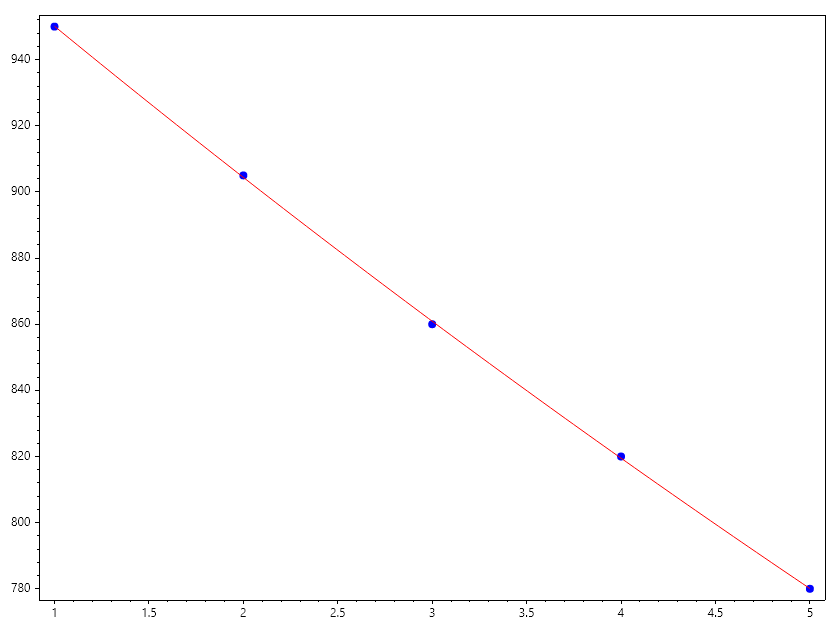
Linearization for Exponential Decline

The exponential equation $q = q_i e^{-Dt}$ can be linearized by taking the natural logarithm of both sides:

\ln(q) = \ln(q_i) - D \cdot t

By plotting $\ln(q)$ vs. $t$ , the slope is $-D$ and the intercept is $\ln(q_i)$ .

Practical Example:

Example 2C#

// Data: t (months), q (STB/day)
double[] t = [1, 2, 3, 4, 5];
double[] q = [950, 905, 860, 820, 780];
double[] Lnq = [..q.Select(Log)];
var p = Polyfit(t, Lnq, 1);
double D = -p[0];
double q_i = Exp(p[1]);
Console.WriteLine($"D = {D} per month");
Console.WriteLine($"q_i = {q_i} STB/day");
double[] T = Linspace(t[0], t[^1]);
double[] Q = [.. T.Select(t => q_i * Exp(-D*t))];
Scatter(t, q, "fob"); HoldOn();
Plot(T, Q, "r"); HoldOff();
SaveAs("Exponential_Fit.png");

OutputFrom the book

D = 0.049296673326352236 per month
q_i = 998.1220221050729 STB/day

Linearization for Harmonic Decline (:math:`b=1`)

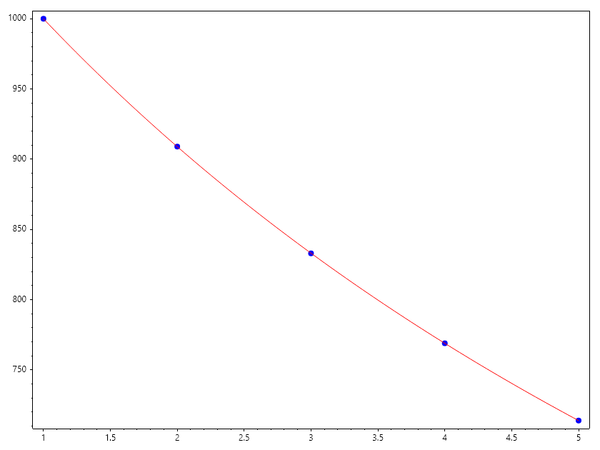
The harmonic equation $q = q_i / (1 + D_i t)$ is linearized by taking the reciprocal of the rate:

\frac{1}{q} = \frac{1}{q_i} + \left(\frac{D_i}{q_i}\right) \cdot t

By plotting $1/q$ vs. $t$ , the slope is $D_i/q_i$ and the intercept is $1/q_i$ .

Practical Example:

Example 3C#

double[] t = [1, 2, 3, 4, 5];
double[] q = [1000, 909, 833, 769, 714];
double[] iq = [.. q.Select(q=>1/q)];
var p = Polyfit(t, iq, 1);
double D = p[0]/p[1];
double q_i = 1/p[1];
Console.WriteLine($"D = {D} per month");
Console.WriteLine($"q_i = {q_i} STB/day");
double[] T = Linspace(t[0], t[^1]);
double[] Q = [.. T.Select(t => q_i /(1 + D*t))];
Scatter(t, q, "fob"); HoldOn();
Plot(T, Q, "r"); HoldOff();
SaveAs("Harmonic_Fit.png");

OutputFrom the book

D = 0.11128058359645096 per month
q_i = 1111.2494708361232 STB/day

Hyperbolic Decline (:math:`0 < b < 1`)

The most common decline type. The decline rate itself decreases over time.

Numerical Example:

Given:

$q_i = 1500 \, \text{Mscf/day}$

$D_i = 0.10 \, \text{per month}$

$b = 0.5$

q(t) = \frac{1500}{(1 + 0.5 \cdot 0.1 \cdot 12)^{1/0.5}} = \frac{1500}{(1.6)^2} = 585.9 \, \text{Mscf/day}

Example 4C#

double qi = 1500;
double Di = 0.10;
double b = 0.5;
double t = 12;
double q_t = qi / Pow(1 + b * Di * t, 1 / b);
Console.WriteLine($"Hyperbolic Rate = {q_t:F2} Mscf/day");

OutputFrom the book

Hyperbolic Rate = 585.94 Mscf/day

Linearization for Hyperbolic Decline

Hyperbolic decline ( $0 < b < 1$ ) cannot be fully linearized with simple variables because of the $b$ exponent. Instead, we linearize the Loss Ratio ( $1/D$ ), defined as $a = q / (dq/dt)$ :

\frac{q}{dq/dt} = \frac{1}{D_i} + b \cdot t

To solve this, we compute the derivative of production over time, plot the loss ratio vs. $t$ , and find $b$ (slope) and $1/D_i$ (intercept).

Practical Example:

Example 5C#

// Loss Ratio (a) calculated from historical data
double[] t = { 1, 2, 3, 4, 5 };
double[] loss_ratio = { 10.5, 11.0, 11.5, 12.0, 12.5 };

Cumulative Production and EUR

To calculate the Estimated Ultimate Recovery (EUR), we integrate the rate over time until a limit rate ( $q_{limit}$ ) is reached.

For Exponential Decline:

G_p = \frac{q_i - q(t)}{D}

Example 6C#

double qi = 1000;
double q_limit = 50; // Economic limit
double D = 0.05;
double EUR = (qi - q_limit) / D;
Console.WriteLine($"EUR (Exponential) = {EUR:F2} STB");

OutputFrom the book

EUR (Exponential) = 19000.00 STB

Computing the Exponential Model Decline Rate

Using the given data

Example 7C#

double[] t = [0, 10, 20, 30, 40, 50, 60, 70, 80, 90];
double[] qt = [double.NaN, 990.05, 980.20, 970.45, 960.78, 951.23, 941.76, 932.39, 923.12, 913.93];

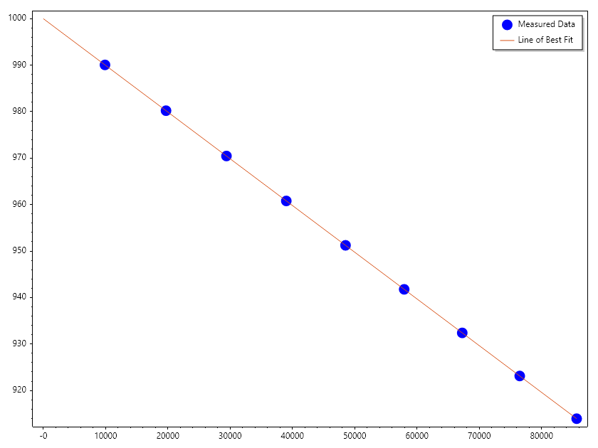
Solution - 1. Compute the commulative production Np - 2. Plot qt versus Np and measure the slope and intercept - 3. intercept is the $q_i$ and slope is the $D$

Example 8C#

double[] t = [0, 10, 20, 30, 40, 50, 60, 70, 80, 90];
double[] qt = [double.NaN, 990.05, 980.20, 970.45, 960.78, 951.23, 941.76, 932.39, 923.12, 913.93];
// Compute Cumulative
double[] Np = Zeros(t.Length);
for (int i = 1; i < t.Length; i++)
    Np[i] = Np[i-1] + qt[i]*(t[i] - t[i-1]);
// Compute Slope and Intercept
double[] coeffs = Polyfit(Np[1..], qt[1..], 1);
// Plot
Scatter(Np[1..], qt[1..], "fob", 15); HoldOn();
Plot(Np, [.. Np.Select(np => Polyval(coeffs, np))]); HoldOff();
Legend(["Measured Data", "Line of Best Fit"]);
SaveAs("Decline_Curve_Fitting.png");
// Print Result
Console.WriteLine($"D = {coeffs[0]}");
Console.WriteLine($"q_i = {coeffs[1]}");

OutputFrom the book

D = -0.0010050369357366175
q_i = 999.9999607852839

Data with Shutdown

Given this production history with shutdown

Example 9C#

double[] qt = [990, 0, 980, 970, 0, 961, 951, 942, 0, 0, 932, 923, 914, 905];
double[] t = [10, 20, 30, 40, 50, 60, 70, 80, 90, 100, 110, 120, 130, 140];
double[] Np = Zeros(t.Length);
for (int i = 1; i < t.Length; i++)
    Np[i] = Np[i-1] + qt[i]*(t[i] - t[i-1]);
//filter
Np = [.. Np.Where((np, i) => qt[i] > 0)];
qt = [.. qt.Where((q, i) => qt[i] > 0)];
t = [.. t.Where((t, i) => qt[i] > 0)];
var p = Polyfit(Np, qt, 1);
// Plot
Scatter(Np[1..], qt[1..], "fob", 15); HoldOn();
Plot(Np, [.. Np.Select(np => Polyval(p, np))]); HoldOff();
Legend(["Measured Data", "Line of Best Fit"]);
SaveAs("Decline_Curve_Fitting.png");
// Print Result
Console.WriteLine($"D = {p[0]}");
Console.WriteLine($"q_i = {p[1]}");

OutputFrom the book

⚠️ Runtime Error: Index was outside the bounds of the array.

Assuming an exponential decline model

1. Plot the t vs Q
2. delete the zeros and the corresponding times and adjust the time to delete the shutdown time
3. using exponential fit, estimate the intial rate and the decline rate.

Using the second approach of cumulative versus rate

4. Compute Cummulative production
5. Plot the production rate versus cumulative production
6. Delete the zero rates and the corresponding cumulative production
7. using linear fit. estimete the initial rate and the decline rate.