Interpolation by Polynomial — SepalSolver

Interpolation via Polynomial Fitting

While standard interpolation (like linear or Hermite) forces a curve to pass through every single data point, Polynomial Fit Interpolation uses a global model to approximate the data. This is particularly useful when you have many data points that might contain noise, or when you want a single mathematical expression to describe the entire dataset.

1. The Strategy

Modeling: Use Polyfit to find the coefficients of a polynomial of degree :math:N that best represents the data.
Estimation: Use Evaluate to calculate the value of that polynomial at any arbitrary point $x$ .

2. Global vs. Local Interpolation

Example 1C#

// Measured data points
double[] X = [0.0, 1.0, 2.0, 3.0, 4.0], Y = [1.2, 1.9, 4.3, 8.8, 17.1];
// Stage 1: Fit a quadratic (N=2) to create the model
double[] model = Polyfit(X, Y, 2);
// Stage 2: Interpolate at a point between 2.0 and 3.0
double[] x = Linspace(0, 4);
double evaluator(double x) => Polyval(model, x);
double[] estimate = [.. x.Select(evaluator)];
Scatter(X, Y, "fob", 12); HoldOn();
Plot(x, estimate, "r"); HoldOff();
SaveAs("Polynomial_Interpolation_Ex1.png");

OutputFrom the book

Examples

.. Admonition:: Example 1 : Signal Denoising and Prediction

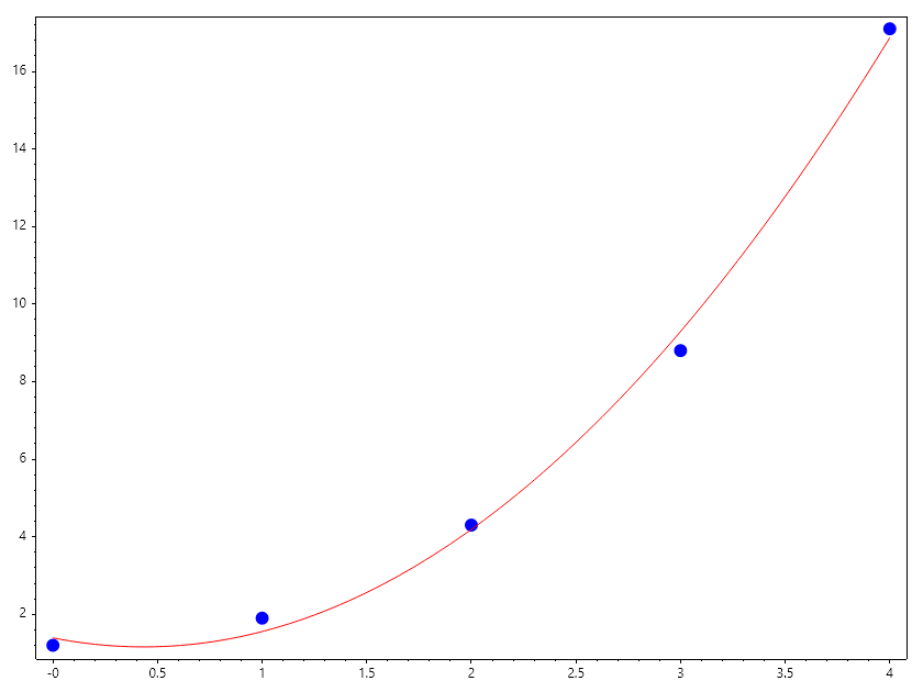
In sensor applications, individual readings often jump due to electronic noise.By fitting a low-degree polynomial to a window of data, you "smooth out" the noise.You can then interpolate to find values at high-frequency time steps that the sensor didn't actually record.

Example 2C#

double[] time = [0.1, 0.2, 0.3, 0.4, 0.5], volts = [1.02, 1.05, 1.01, 1.08, 1.04];
// Fit a line (N=1) to find the steady trend
double[] trend = Polyfit(time, volts, 1);
// Interpolate at a point in the middle
double midVoltage = Polyval(trend, 0.25);
// Print out result
Console.WriteLine($" midvoltage = {midVoltage}");

OutputFrom the book

midvoltage = 1.0365000000000002

.. Admonition:: Example 2 : Structural Deformation Mapping

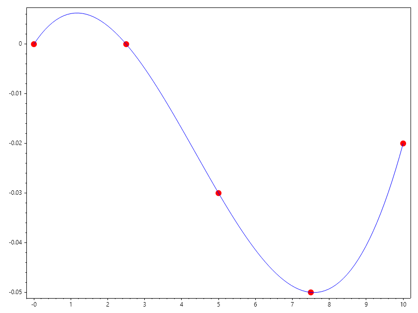
If you measure the deflection of a beam at 5 specific locations, a polynomial fit of degree 3 or 4 can describe the continuous "shape" of the beam.You can then use this model to interpolate the deflection at any other point along the beam's length.

Example 3C#

double[] x = Linspace(0,10, 5), y = [0, 0, -0.03, -0.05, -0.02];
ColVec xc = x, yc = y;
double[] coeffs = Polyfit(x, y, 3); //degree2
ColVec xq = Linspace(0, 10);
ColVec yq = Arrayfun(x => Polyval(coeffs, x), xq);
Scatter(xc, yc, "for", 12); HoldOn();
Plot(xq, yq, "b"); HoldOff();
SaveAs("Polynomial_Interpolation_Ex3.png");

OutputFrom the book

Exercise: Choosing the Degree

Task: Determine which degree :math:N is most appropriate for the data and evaluate.

Example 4C#

double[] x = [1, 2, 3, 4, 5, 6], y = [2.1, 4.2, 5.9, 8.1, 10.3, 11.9];
Looks like y = 2x//
Task: Fit a linear model and interpolate at x = 3.5
int degree = ____;
double[] p = Polyfit(x, y, degree);
double result = Polyval(p, 3.5);
// Expected: Roughly 7.0
Console.WriteLine($"Result at 3.5: :math:`{result}`");

Multivariate Application

The idea of using polynomial fits can be extended to multiple dimensions. For example, if you have data points in 2D space (x, y) with corresponding values z, you can fit a polynomial surface to approximate z as a function of x and y. This is particularly useful in fields like geostatistics or thermodynamic property evaluation, where you want to model complex surfaces based on scattered data.

.. Admonition:: Example 4 : Thermodynamic Property Estimation

Example 5C#

double[] Temperature = [1000, 1100, 1200, 1300, 1400, 1500, 1600, 1800, 2000],
    Pressure = [0.01, 0.02, 0.03, 0.04, 0.05, 0.06];
double[,] SpecificVolume = new double[,]
{
    {58.758, 29.379, 19.586, 14.689, 11.751, 9.7927},
    {63.373, 31.686, 21.124, 15.843, 12.674, 10.562},
    {67.988, 33.994, 22.663, 16.997, 13.598, 11.331},
    {72.604, 36.302, 24.201, 18.151, 14.521, 12.101},
    {77.219, 38.61,  25.74,  19.305, 15.444, 12.87},
    {81.834, 40.917, 27.278, 20.459, 16.367, 13.639},
    {86.45,  43.225, 28.817, 21.613, 17.29,  14.409},
    {95.68,  47.84,  31.894, 23.92,  19.136, 15.947},
    {104.91, 52.455, 34.97,  26.228, 20.982, 17.485}
};
// Fit a 2nd degree polynomial surface
(Matrix Tmesh, Matrix Pmesh) = Meshgrid(Temperature, Pressure);
Matrix SVmesh = SpecificVolume;
double[] x = [.. Tmesh], y = [.. Pmesh], xy = [.. Tmesh.Times(Pmesh)], z = [.. SVmesh];
// Task: Make the Matrix A with the cross term included
List<ColVec> A = [Ones(x.Length), x, y, xy];
// Solve for the coefficients using Least Squares
var coeffs = Mldivide(A, z);
// Interpolate at T = 1350K, P = 0.0373MPa
double T = 1350, P = 0.0373;
double sv = coeffs[0] + coeffs[1] * T + coeffs[2] * P + coeffs[3] * T * P;
Console.WriteLine("Interpolation by Polynomial Fitting");
Console.WriteLine($"Specific volume at T = {T} and P = {P} is {sv}");
// Note that this is different from what we obtained from bilinear interpolation
sv = Interp2(Temperature, Pressure, SpecificVolume, T, P);
Console.WriteLine("Interpolation by Bilinear Interpolation");
Console.WriteLine($"Specific volume at T = {T} and P = {P} is {sv}");
// We can obtain the same result as intepolation of we select the region used by linear interpolation
Tmesh = Tmesh[3..5, 2..4]; Pmesh = Pmesh[3..5, 2..4]; SVmesh = SVmesh[3..5, 2..4];
x = [.. Tmesh]; y = [.. Pmesh]; xy = [.. Tmesh.Times(Pmesh)]; z = [.. SVmesh];
A = [Ones(x.Length), x, y, xy]; coeffs = Mldivide(A, z);
sv = coeffs[0] + coeffs[1] * T + coeffs[2] * P + coeffs[3] * T * P;
Console.WriteLine("Interpolation by Polynomial Fitting-Using Narrow Region");
Console.WriteLine($"Specific volume at T = {T} and P = {P} is {sv}");

double[] Temperature = [1000, 1100, 1200, 1300, 1400, 1500, 1600, 1800, 2000],
    Pressure = [0.01, 0.02, 0.03, 0.04, 0.05, 0.06];
double[,] SpecificVolume = new double[,]
{
    {58.758, 29.379, 19.586, 14.689, 11.751, 9.7927},
    {63.373, 31.686, 21.124, 15.843, 12.674, 10.562},
    {67.988, 33.994, 22.663, 16.997, 13.598, 11.331},
    {72.604, 36.302, 24.201, 18.151, 14.521, 12.101},
    {77.219, 38.61,  25.74,  19.305, 15.444, 12.87},
    {81.834, 40.917, 27.278, 20.459, 16.367, 13.639},
    {86.45,  43.225, 28.817, 21.613, 17.29,  14.409},
    {95.68,  47.84,  31.894, 23.92,  19.136, 15.947},
    {104.91, 52.455, 34.97,  26.228, 20.982, 17.485}
};

// Fit a 2nd degree polynomial surface
(Matrix Tmesh, Matrix Pmesh) = Meshgrid(Temperature, Pressure);
Matrix SVmesh = SpecificVolume;
double[] x = [.. Tmesh], y = [.. Pmesh], xy = [.. Tmesh.Times(Pmesh)], z = [.. SVmesh];

// Task: Make the Matrix A with the cross term included
List<ColVec> A = [Ones(x.Length), x, y, xy];

// Solve for the coefficients using Least Squares
var coeffs = Mldivide(A, z);

// Interpolate at T = 1350K, P = 0.0373MPa
double T = 1350, P = 0.0373;
double sv = coeffs[0] + coeffs[1] * T + coeffs[2] * P + coeffs[3] * T * P;
Console.WriteLine("Interpolation by Polynomial Fitting");
Console.WriteLine($"Specific volume at T = {T} and P = {P} is {sv}");

// Note that this is different from what we obtained from bilinear interpolation
sv = Interp2(Temperature, Pressure, SpecificVolume, T, P);
Console.WriteLine("Interpolation by Bilinear Interpolation");
Console.WriteLine($"Specific volume at T = {T} and P = {P} is {sv}");

// We can obtain the same result as intepolation of we select the region used by linear interpolation
Tmesh = Tmesh[3..5, 2..4]; Pmesh = Pmesh[3..5, 2..4]; SVmesh = SVmesh[3..5, 2..4];
x = [.. Tmesh]; y = [.. Pmesh]; xy = [.. Tmesh.Times(Pmesh)]; z = [.. SVmesh];
A = [Ones(x.Length), x, y, xy]; coeffs = Mldivide(A, z);
sv = coeffs[0] + coeffs[1] * T + coeffs[2] * P + coeffs[3] * T * P;
Console.WriteLine("Interpolation by Polynomial Fitting-Using Narrow Region");
Console.WriteLine($"Specific volume at T = {T} and P = {P} is {sv}");

OutputFrom the book

Interpolation by Polynomial Fitting
Specific volume at T = 1350 and P = 0.0373 is 28.053581185031376
Interpolation by Bilinear Interpolation
Specific volume at T = 1350 and P = 0.0373 is 20.413475
Interpolation by Polynomial Fitting-Using Narrow Region
Specific volume at T = 1350 and P = 0.0373 is 20.413475000000012