Hemite Spline — SepalSolver

Hermite Interpolation

Hermite Interpolation is a method of interpolating data points that accounts for not only the values of the function but also the values of its derivatives. While standard linear or polynomial interpolation only ensures the curve passes through the points $(x_i, y_i)$ . Hermite interpolation ensures the curve matches the "slope"(tangent) at those points as well. This results in a much smoother and more physically realistic transition between points, particularly in motion planning or structural deflection models where velocity or tangency must be continuous.

1. The Cubic Hermite Spline

The most common form is the Cubic Hermite Spline. For a single interval between $x_0$ and $x_1$ the interpolant is a third-degree polynomial.To construct it, we need four pieces of information: The starting and ending values: $y_0$ and $y_1$ The starting and ending derivatives (slopes): $y'_0$ and $y'_1$

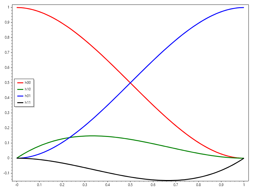
The resulting curve is expressed using Hermite Basis Functions, which act as weights for the coordinates and the slopes.

Example 1C#

ColVec t = Linspace(0, 1), t2 = t.Pow(2), t3 = t.Pow(3);
ColVec h00 = 2 * t3 - 3 * t2 + 1, h10 = t3 - 2 * t2 + t,
       h01 = -2 * t3 + 3 * t2, h11 = t3 - t2;
Plot(t, h00, "r", 3); HoldOn();
Plot(t, h10, "g", 3);
Plot(t, h01, "b", 3);
Plot(t, h11, "k", 3); HoldOff();
Legend(["h00", "h10", "h01", "h11"], MiddleLeft);
SaveAs("hermite_modes.png");

OutputFrom the book

2. Implementation in SepalSolver

In SepalSolver, Hermite interpolation is often used when the user provides a "slope vector" alongside their dataset. This is common in trajectory generation where you know where a robot should be and how fast it should be moving at that specific moment.

Example 2C#

double[] x = [0.0, 1.0]; 
double[] y = [0.0, 10.0];
double[] dy = [0.0, 0.0]; // Zero velocity at start and end
// Estimate value at x = 0.5
double xq = 0.5;
// Manually implementing Hermite interpolation
double x0 = x[0], x1 = x[1], y0 = y[0], y1 = y[1], m0 = dy[0], m1 = dy[1];
double dx = x1 - x0, t = (xq - x0) / dx, t2 = t * t, t3 = t2 * t;
double h00 = 2 * t3 - 3 * t2 + 1, 
       h10 = t3 - 2 * t2 + t,
       h01 = -2 * t3 + 3 * t2, 
       h11 = t3 - t2;
double result = h00 * y0 + h10 * dx * m0 + h01 * y1 + h11 * dx * m1;
// Because slopes are 0, this creates an S-curve rather than a straight line
Console.WriteLine($"Smooth transition value: {result}");

OutputFrom the book

Smooth transition value: 5

Examples

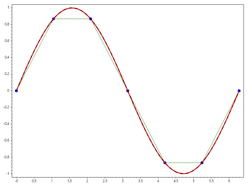
.. Admonition:: Example 1 : Compare Linear and Hermite interpolation for sparsely compited sin(x)

If sin(x) is give at 7 points between $0$ and $\pi$ . Interpolate for sin(x) for 100 points between $0$ and $\pi$ using linear and hermite spline and compare the plots.

Example 3C#

// Using linear interpolation
ColVec x = Linspace(0, 2*pi, 7), s = Sin(x);
ColVec xq = Linspace(0, 2*pi), sq = Interp1(x, s, xq);
Scatter(x, s, "fob", 10); HoldOn();
Plot(xq, sq, "g");
// using hermite interpolation
int j = 1;
ColVec c = Cos(x);
ColVec sh = Zeros(xq.Numel);
for (int i = 0; i < xq.Numel; i++)
{
    while (xq[i] > x[j]) j++;
    double x0 = x[j-1], x1 = x[j], y0 = s[j-1], y1 = s[j], m0 = c[j-1], m1 = c[j];
    double dx = x1 - x0, t = (xq[i] - x0) / dx, t2 = t * t, t3 = t2 * t;
    double h00 = 2 * t3 - 3 * t2 + 1, 
           h10 = t3 - 2 * t2 + t,
           h01 = -2 * t3 + 3 * t2, 
           h11 = t3 - t2;
    sh[i] = h00 * y0 + h10 * dx * m0 + h01 * y1 + h11 * dx * m1;
}
Plot(xq, sh, "r", 3);
Plot(xq, Sin(xq), "--k", 2); HoldOff();
SaveAs("hermite_vs_linear.png");

OutputFrom the book

.. Admonition:: Example 2 :

If a robot moves from point A to point B, a linear path causes an abrupt change in velocity at the corners. By using Hermite interpolation and specifying the desired entry/exit velocity vectors, we create a path that the robot can follow without stopping or jerking.

Example 4C#

double[] t = [0, 5, 10];    // Time
double[] pos = [0, 20, 50]; // Position
double[] vel = [0, 10, 0];  // Specific velocities at those times

Key Difference: Hermite vs. Cubic Spline

Feature	Hermite Interpolation	Cubic Spline
Input Requirements	Requires $y$ and $y'$ (slopes)	Requires only $y$
Local Control	Changing one slope only affects the two adjacent segments	Changing one point can affect the entire curve
Complexity	Mathematically simpler (local calculation)	Requires solving a system of equations (global)

Exercise: Animation of Slope Impact

Task: Observe how changing the slope $dy$ at the first point affects the plot of the function.

Example 5C#

//define hemitespline function
double[] HermiteFun(double[] x, double[] y, double[] dy, double[] xq)
{
    double[] yq = new double[xq.Length];
    int j = 1;
    for (int i = 0; i < xq.Length; i++)
    {
        while (xq[i] > x[j]) j++;
        double x0 = x[j-1], x1 = x[j], y0 = y[j-1], y1 = y[j], m0 = dy[j-1], m1 = dy[j];
        double dx = x1 - x0, t = (xq[i] - x0) / dx, t2 = t * t, t3 = t2 * t;
        double h00 = 2 * t3 - 3 * t2 + 1,
               h10 = t3 - 2 * t2 + t,
               h01 = -2 * t3 + 3 * t2,
               h11 = t3 - t2;
        yq[i] = h00 * y0 + h10 * dx * m0 + h01 * y1 + h11 * dx * m1;
    }
    return yq;
}
// define x and y
double[] x = [0, 1];
double[] y = [0, 0];
// start with this slope
double[] dy = [-1, 1];
// define querry points
double[] xq = Linspace(0, 1);
double[] yq = HermiteFun(x, y, dy, xq);
// plot the result.
var plt = Plot(xq, yq, Linewidth: 2);
Axis([0, 1, -0.3, 0.2]);
// set up animation function
byte[] animfun(int i)
{
    dy[0] = Sin(pi + i * 0.02*pi);           // increase the starting slope
    plt.Ydata = HermiteFun(x, y, dy, xq);    // update interpolated values
    return GetFrame();                       //  return the frame
}
// Animate the plot
AnimationMaker(animfun, "Impact_of_changing_slope_at_x_0.gif", 30, 100);

//define hemitespline function
double[] HermiteFun(double[] x, double[] y, double[] dy, double[] xq)
{
    double[] yq = new double[xq.Length];
    int j = 1;
    for (int i = 0; i < xq.Length; i++)
    {
        while (xq[i] > x[j]) j++;

double x0 = x[j-1], x1 = x[j], y0 = y[j-1], y1 = y[j], m0 = dy[j-1], m1 = dy[j];
        double dx = x1 - x0, t = (xq[i] - x0) / dx, t2 = t * t, t3 = t2 * t;

double h00 = 2 * t3 - 3 * t2 + 1,
               h10 = t3 - 2 * t2 + t,
               h01 = -2 * t3 + 3 * t2,
               h11 = t3 - t2;
        yq[i] = h00 * y0 + h10 * dx * m0 + h01 * y1 + h11 * dx * m1;
    }
    return yq;
}

// define x and y
double[] x = [0, 1];
double[] y = [0, 0];

// start with this slope
double[] dy = [-1, 1];

// define querry points
double[] xq = Linspace(0, 1);
double[] yq = HermiteFun(x, y, dy, xq);

// plot the result.
var plt = Plot(xq, yq, Linewidth: 2);
Axis([0, 1, -0.3, 0.2]);

// set up animation function
byte[] animfun(int i)
{
    dy[0] = Sin(pi + i * 0.02*pi);           // increase the starting slope
    plt.Ydata = HermiteFun(x, y, dy, xq);    // update interpolated values
    return GetFrame();                       //  return the frame
}

// Animate the plot
AnimationMaker(animfun, "Impact_of_changing_slope_at_x_0.gif", 30, 100);

</example 4>

.. Admonition:: Example 5 : Using Hermite Spline as Sin Approximator

Lets use table of Sine and Cosine at 15 degrees interval given in table

Angle (°)	Sine ( $\sin$ )	Cosine ( $\cos$ )
0°	$0$	$1$
15°	$\cfrac{\sqrt{6} - \sqrt{2}}{4}$	$\cfrac{\sqrt{6} + \sqrt{2}}{4}$
30°	$\cfrac{1}{2}$	$\cfrac{\sqrt{3}}{2}$
45°	$\cfrac{\sqrt{2}}{2}$	$\cfrac{\sqrt{2}}{2}$
60°	$\cfrac{\sqrt{3}}{2}$	$\cfrac{1}{2}$
75°	$\cfrac{\sqrt{6} + \sqrt{2}}{4}$	$\cfrac{\sqrt{6} - \sqrt{2}}{4}$
90°	$1$	$0$

Example 6C#

// compute square roots of 2 and 3;
double sqrt2 = Sqrt(2), sqrt3 = Sqrt(3);
// define arrays of angle, sine and cosines
double[] Sines = [0, sqrt2*(sqrt3-1)/4, 0.5, sqrt2/2, sqrt3/2, sqrt2*(sqrt3+1)/4, 1];
double[] Cosines = [1, sqrt2*(sqrt3+1)/4, sqrt3/2, sqrt2/2, 0.5, sqrt2*(sqrt3-1)/4, 0];
double SineByHermite(double a)
{
    double da = 15;
    int i = (int)(a/da);
    double t = (a - i*da)/da;
    if (t == 0)
        return Sines[i];
    else
    {
        double t2 = t * t, t3 = t2 * t, dx = da*pi/180;
        double y0 = Sines[i], y1 = Sines[i+1], m0 = Cosines[i], m1 = Cosines[i+1];
        double h00 = 2 * t3 - 3 * t2 + 1,  h10 = t3 - 2 * t2 + t,
               h01 = -2 * t3 + 3 * t2,  h11 = t3 - t2;
        return h00 * y0 + h10 * dx * m0 + h01 * y1 + h11 * dx * m1;
    }
}
double[] x = [.. Rand(20).Select(a => 80*a+10)];
Console.WriteLine("""
      Angle  |  Sineapprox  |    Sine
    ---------+--------------+-------------
    """);
foreach (double a in x)
    Console.WriteLine($"""
          {a:F2}  |   {SineByHermite(a):F6}   |  {Sin(a*pi/180):F6}
        """);

// compute square roots of 2 and 3;
double sqrt2 = Sqrt(2), sqrt3 = Sqrt(3);

// define arrays of angle, sine and cosines
double[] Sines = [0, sqrt2*(sqrt3-1)/4, 0.5, sqrt2/2, sqrt3/2, sqrt2*(sqrt3+1)/4, 1];
double[] Cosines = [1, sqrt2*(sqrt3+1)/4, sqrt3/2, sqrt2/2, 0.5, sqrt2*(sqrt3-1)/4, 0];

double SineByHermite(double a)
{
    double da = 15;
    int i = (int)(a/da);
    double t = (a - i*da)/da;
    if (t == 0)
        return Sines[i];
    else
    {

double t2 = t * t, t3 = t2 * t, dx = da*pi/180;
        double y0 = Sines[i], y1 = Sines[i+1], m0 = Cosines[i], m1 = Cosines[i+1];
        double h00 = 2 * t3 - 3 * t2 + 1,  h10 = t3 - 2 * t2 + t,
               h01 = -2 * t3 + 3 * t2,  h11 = t3 - t2;
        return h00 * y0 + h10 * dx * m0 + h01 * y1 + h11 * dx * m1;
    }
}

double[] x = [.. Rand(20).Select(a => 80*a+10)];
Console.WriteLine("""
      Angle  |  Sineapprox  |    Sine
    ---------+--------------+-------------
    """);
foreach (double a in x)
    Console.WriteLine($"""
          {a:F2}  |   {SineByHermite(a):F6}   |  {Sin(a*pi/180):F6}
        """);

OutputFrom the book

  Angle  |  Sineapprox  |    Sine
---------+--------------+-------------
  22.47  |   0.382216   |  0.382220
  49.22  |   0.757171   |  0.757178
  34.61  |   0.568044   |  0.568049
  39.39  |   0.634616   |  0.634623
  76.86  |   0.973822   |  0.973824
  81.41  |   0.988768   |  0.988780
  80.35  |   0.985833   |  0.985843
  19.16  |   0.328197   |  0.328200
  12.59  |   0.217959   |  0.217960
  38.53  |   0.622888   |  0.622895
  42.79  |   0.679328   |  0.679330
  20.26  |   0.346344   |  0.346347
  22.28  |   0.379171   |  0.379176
  25.29  |   0.427126   |  0.427129
  47.94  |   0.742429   |  0.742432
  64.80  |   0.904815   |  0.904823
  23.18  |   0.393599   |  0.393604
  31.18  |   0.517792   |  0.517793
  17.09  |   0.293856   |  0.293857
  43.92  |   0.693713   |  0.693713