Polynomial Fitting — SepalSolver

Polynomial Fitting (Polyfit)

In engineering and data science, we often encounter discrete data points that represent a physical process. Polynomial Fitting is the mathematical technique used to find a continuous function—specifically a polynomial—that minimizes the discrepancy between the curve and the observed data. In SepalSolver, we use the Least Squares approach to determine these coefficients.

1. Mathematical Objective

The goal of Polyfit is to find a set of coefficients for a polynomial of degree $N$ :, $P(x) = a_0 x^N + a_1 x^{N-1} + \dots + a_N$ such that the sum of the squares of the residuals (the vertical distance between the data points and the curve) is minimized.

2. Coefficient Order

Note that while the internal math often builds from the constant term up, SepalSolver returns the resulting double[] array in descending order. This means the first element in the array is the coefficient for the highest power $x^N$ .

Examples

.. Admonition:: Example 1 : Fitting a Perfect Quadratic

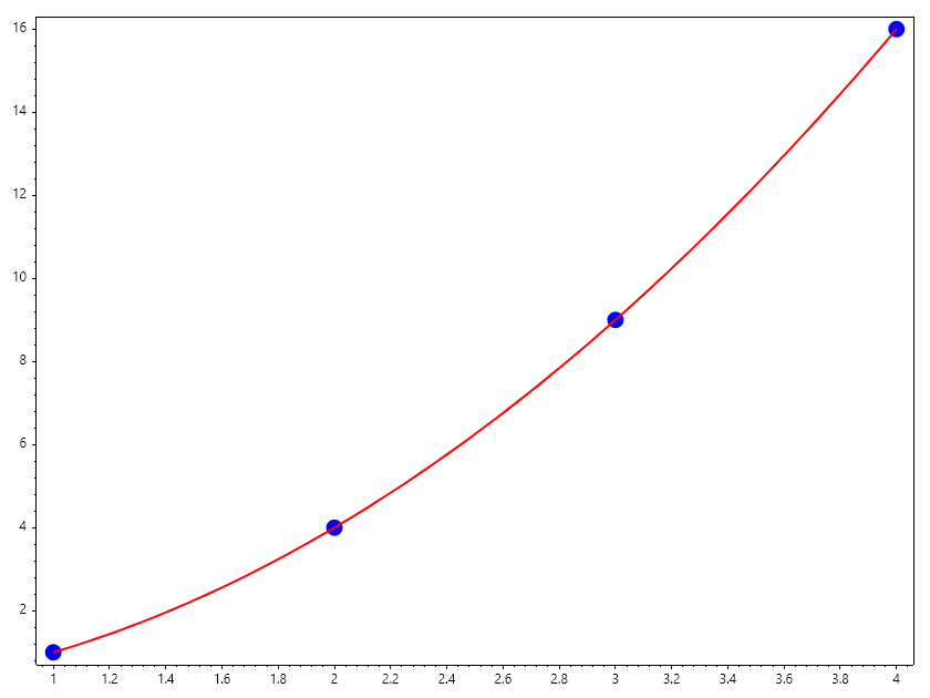
If our data follows a perfect square relationship, such as $y = x^2$ , we expect Polyfit to return coefficients that reflect $1x^2 + 0x + 0$ . In this example, we fit a degree $N=2$ polynomial to a set of coordinates.

Example 1C#

// Define data points
double[] X = [1, 2, 3, 4]; 
double[] Y = [1, 4, 9, 16]; 
int N = 2;
// Perform the fit
double[] coefficients = Polyfit(X, Y, N);
// Output: 1, 0, 0 (representing 1x^2 + 0x + 0)
Console.WriteLine($"Coefficients: [{string.Join(", ", coefficients.Select(n => n.ToString("F4")))}]");
// Plotting the results
Scatter(X, Y, "fob", 15); HoldOn();
double[] x = Linspace(1, 4);
double[] y = [..x.Select(x => Polyval(coefficients, x))];
Plot(x, y, "r", Linewidth: 2); HoldOff();
SaveAs("Polyfit_Example1.png");

OutputFrom the book

Coefficients: [1.0000, 0.0000, 0.0000]

.. Admonition:: Example 2 : Linear Regression from Sensor Data

Imagine you are testing a linear spring. You record the force $Y$ applied at various displacements $X$ . By fitting a degree $N=1$ polynomial, you can find the spring constant $k$ , which corresponds to the first coefficient in the returned array.

Example 2C#

double[] X = [0.1, 0.2, 0.3, 0.4];     // Displacement
double[] Y = [10.2, 20.1, 29.9, 40.2]; // Force
// Fit a line: P(x) = a0*x + a1
double[] p = Polyfit(X, Y, 1);
Console.WriteLine($"Spring Constant k: {p[0]} N/m");

OutputFrom the book

Spring Constant k: 99.79999999999995 N/m

.. Admonition:: Example 3 : Handling Noise in Experimental Data

Real-world data is rarely perfect. When data points are "noisy," fitting a lower-degree polynomial acts as a filter, capturing the general trend without being distracted by individual measurement errors.

Example 3C#

double[] X = [1, 2, 3, 4, 5]; 
double[] Y = [2.1, 3.9, 6.2, 8.1, 9.8]; // Roughly y = 2x
// Even if we fit a degree 2, the leading coefficient should be near zero
double[] p = Polyfit(X, Y, 2);
Console.WriteLine($"Quadratic term (should be small): {p[0]}");

OutputFrom the book

Quadratic term (should be small): -0.04285714285714366

Usage Warning

Ensure that the length of arrays $X$ and $Y$ are identical. Additionally, to find a unique solution for a degree $N$ polynomial, you must provide at least $N+1$ data points. Providing fewer points will result in an underdetermined system and numerical instability. It is also important to choose the correct degree of the polynomial to get a good fit. Overfitting can occur if the degree is too high, while underfitting can happen if the degree is too low.

.. Admonition:: Example 4 : Underfitting Problem

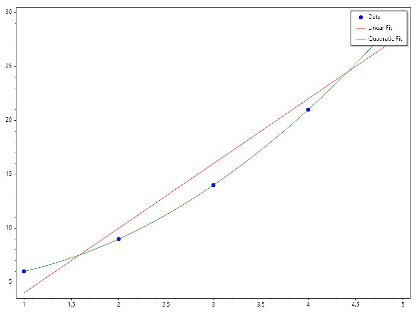
In this example, we compare a linear and quaradtic fit for the same data. showing the importance of choosing the right degree for the fitting.

Example 4C#

// Example of polynomial fitting
double[] x = [1, 2, 3, 4, 5], y = [6, 9, 14, 21, 30];
Scatter(x, y, "fob"); HoldOn();
double[] xp = Linspace(1, 5);
double[] fit1 = Polyfit(x, y, 1);
double[] yp1 = [.. xp.Select(x => Polyval(fit1, x))];
Plot(xp, yp1, "r");
Console.WriteLine($"""
    Linear fit : [{string.Join(",", fit1)}] 
    Residual: {yp1.Zip(y, (l, m) => Pow(l-m, 2)).Sum()}
    """);
double[] fit2 = Polyfit(x, y, 2);
double[] yp2 = [.. xp.Select(x => Polyval(fit2, x))];
Plot(xp, yp2, "g");
Console.WriteLine($"""
    Quaratic fit : [{string.Join(",", fit2)}] 
    Residual: {yp2.Zip(y, (q, m) => Pow(q-m, 2)).Sum()}
    """);
Legend(["Data", "Linear Fit", "Quadratic Fit"]);
HoldOff();
SaveAs("Polyfit_Example_4.png");

OutputFrom the book

Linear fit : [5.999999999999998,-1.9999999999999942] 
Residual: 1008.4903581267214
Quaratic fit : [1.0000000000000193,-1.2151770273257475E-13,5.000000000000152] 
Residual: 846.5558445323921

Multivariate Polynomial Fitting

In many engineering scenarios, a dependent variable :math:z is influenced by multiple independent variables (e.g., $x$ and $y$ ). This is known as Multivariate Fitting or Surface Fitting. While a standard Polyfit handles a single line, a multivariate fit finds a surface that minimizes the residuals across multiple dimensions.

1.The Mathematical Model

For two variables $x$ and $y$ , a second-order multivariate polynomial takes the form: $z(x, y) = a_0 + a_1x + a_2y + a_3x^2 + a_4xy + a_5y^2$ The "cross term" :math: xy is vital because it accounts for the interaction between the two variables—how the influence of :math:x might change depending on the current value of $y$ .

2.Implementation Logic

In SepalSolver, multivariate fitting is performed by constructing an augmented matrix where each column represents a term in the polynomial expansion(1, $x$ , $y$ , $x^2$ , etc.) and solving the resulting linear system.

Example 5C#

// Data points: (x, y) coordinates and observed z values
double[] x = [0, 1, 2, 0, 1, 2], y = [0, 0, 0, 1, 1, 1], z = [1.1, 2.0, 3.9, 2.2, 3.1, 5.1];
// Fitting for a plane: z = a + bx + cy
// We construct a matrix A where rows are [1, x_i, y_i]
List<ColVec> A = [Ones(x.Length), x, y];
// Solve for coefficients using the Normal Equation (Least Squares)
// A' * A * coeff = A' * z
var coeff = Mldivide(A, z);
Console.WriteLine($"Model: z = {coeff[0]} + {coeff[1]}x + {coeff[2]}y");

OutputFrom the book

Model: z = 0.908333333333332 + 1.4250000000000007x + 1.133333333333334y

Examples

.. Admonition:: Example 1 : Material Stress Analysis The stress( $\sigma$ ) on a component might depend on both Temperature( $T$ ) and Pressure( $P$ ). A multivariate fit allows you to create a "Stress Surface" that can predict failure points at any combination of: math:T and $P$ .

.. Admonition:: Example 2 : Aero-Efficiency Mapping For a wing, the Lift Coefficient( $C_L$ ) is a function of both the Angle of Attack( $\alpha$ ) and the Mach Number( $M$ ). Using multivariate fitting, flight computers can interpolate lift values instantly across the entire flight envelope.

.. Admonition:: Example 3 :

The Antoine equation relates the vapor pressure of a substance to its temperature:

\log_{10}(p) = A - \frac{B}{C + T}

Where: - $p$ = vapor pressure - $T$ = temperature - $A, B, C$ = substance-specific constants

In other to estimate the values of this constants, we express the equation in a linear form

Step 1: Multiplying Both Sides by $(C + T)$

(C + T)\log_{10}(p) = A(C + T) - B

Step 2: Expanding Both Sides

C\log_{10}(p) + T\log_{10}(p) = AC + AT - B

Step 3: Rearranging the terms:

T\log_{10}(p) = A T - C\log_{10}(p) + (AC - B)

This is a linear equation in terms of $T$ and $log10(p)$ , which can be used to estimate the constants $A$ , $B$ , and $C$ via multiple linear regression.

Slope with respect to $T \to A$
Slope with respect to $log10(p) \to -C$
Intercept $\to AC - B$

$A$ , $B$ , and $C$ can then be solved systematically from regression results.

To estimate the parameters $A$ , $B$ , and $C$

T\log_{10}(p) = \alpha T + \beta C\log_{10}(p) + \gamma

Hence: - $A = \alpha$ - $C = -\beta$ - $B = AC-\gamma$

Example 6C#

// Curve Fitting for Antoine Equation [lnP = A - B/(T + C)]
double[] P_Kpa = [3.18, 5.48, 9.45, 16.9, 28.2, 41.9, 66.6, 89.5, 129, 187],
         T_C = [-18.5, -9.5, 0.2, 11.8, 23.1, 32.7, 44.4, 52.1, 63.3, 75.5];
// Convert Temperature to Kelvin, Compute the natural logarithm of Pressure
ColVec T = (ColVec)T_C + 273.15, LogP = Log10((ColVec)P_Kpa);
ColVec TLogP = T.Times(LogP), One = Ones(T_C.Length);
// Multilinear fit
List<ColVec> M = [T, LogP, One];
var x = Mldivide(M, TLogP);
// Extract fitted parameters
double A = x[0], C = -x[1], B = A*C-x[2];
Console.WriteLine($"Fitted Parameters: A = {A:F4}, B = {B:F4}, C = {C:F4}");

OutputFrom the book

Fitted Parameters: A = 6.1681, B = 1170.7321, C = -48.0075

Exercise: Term Expansion

Task: To fit a full quadratic surface $z = a + bx + cy + dxy$ , your matrix A needs four columns. Complete the column assignment for the cross-term $xy$ .

Example 7C#

// Data points
double[] x = [0, 1, 2, 0, 1, 2], y = [0, 0, 0, 1, 1, 1], z = [1.1, 2.0, 3.9, 2.2, 3.1, 5.1];
// Compute the cross term for multivariate polynomial fitting
double[] xy = [..x.Zip(y, (xi, yi) => xi * yi)];
// Task: Make the Matrix A with the cross term included
// Solve for the coefficients using Least Squares