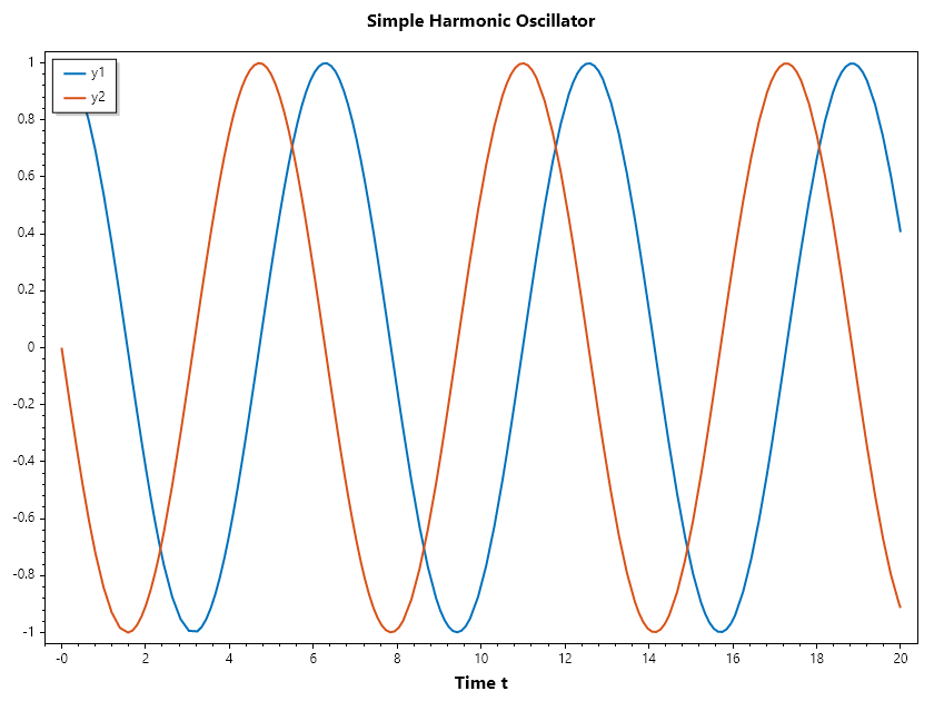
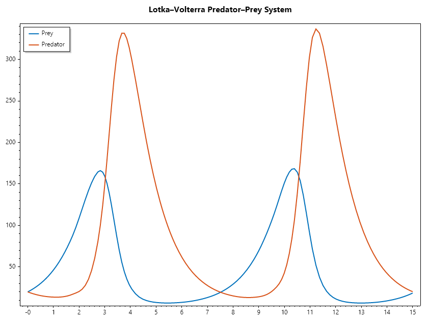
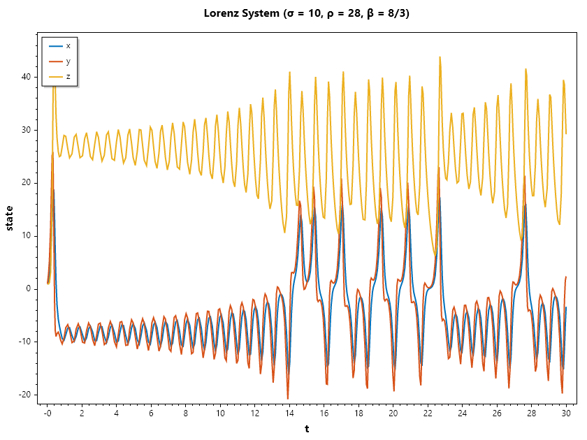
System of First Order Differential Equations — SepalSolver

Introduction

A system of first‑order differential equations involves multiple dependent variables, each with its own derivative, coupled together. Many physical, biological, and engineering models naturally lead to such systems.

Examples:

Predator–prey dynamics(Lotka–Volterra)
Coupled oscillators
Chaotic systems(Lorenz attractor)

SepalSolver provides tools to solve these systems numerically using , just as with single ODEs, but the function signature changes to accept and return arrays.

General Form

A system of $n$ first‑order ODEs can be written as:

\begin{array}{c} \cfrac{dy_1}{dt} = f_1(t, y_1, y_2,\dots, y_n) \\ \cfrac{dy_2}{dt} = f_2(t, y_1, y_2,\dots, y_n) \\ \vdots \\ \cfrac{dy_n}{dt} = f_n(t, y_1, y_2,\dots, y_n) \end{array}

In SepalSolver, this is represented by a function:

Example 1C#

// Define the ODE as a function
double[] dydt(double t, double[] y) => [f1, f2, ..., fn];

where $y$ is the vector of dependent variables.

Examples

These are examples of how to use SepalSolver to solve various systems of first-order ODEs.

.. Admonition:: Example 1 : Simple Harmonic Oscillator

A simple harmonic oscillator can be modeled as a system of first-order ODEs:

\begin{eqnarray} y_1' &= y_2 \\ y_2' &= -y_1 \end{eqnarray}

This represents a simple harmonic oscillator written as a system.

Example 2C#

// Define the ODE as a function
double[] dydt(double t, double[] y) => [ y[1], -y[0] ];
// Initial condition
double[] y0 = [1.0, 0.0];
// Time span
double[] tspan = [0, 20];
// Solve the ODE using Ode45
(ColVec T, Matrix Y) = Ode45(dydt, y0, tspan);
// Plot the results
Plot(T, Y, Linewidth: 2);
Xlabel("Time t");
Legend(["y1", "y2"], UpperLeft);
Title("Simple Harmonic Oscillator");
SaveAs("Simple_Harmonic_Oscillator.png");

OutputFrom the book

.. Admonition:: Example 2 : Lotka–Volterra Predator–Prey

The Lotka–Volterra equations model the dynamics between predator and prey populations. Mathemtically, it is defined as:

\begin{eqnarray} x' &= \alpha x-\beta xy \\ y' &= \delta xy-\gamma y \end{eqnarray}

Example 3C#

// Define the ODE as a function
double alpha = 1.0, beta = 0.01, delta = 0.02, gamma = 1.0;
double[] dydt(double t, double[] y) => [
    alpha * y[0] - beta * y[0] * y[1],
    delta * y[0] * y[1] - gamma * y[1]];
// Initial condition
double[] y0 = [20.0, 20.0];
// Time span
double[] tspan = [0, 15];
// Solve the ODE using Ode45
(ColVec T, Matrix Y) = Ode45(dydt, y0, tspan);
// Plot the results
Plot(T, Y, Linewidth: 2);
Legend(["Prey", "Predator"], UpperLeft);
Title("Lotka–Volterra Predator–Prey System");
SaveAs("Lotka_Volterra_Predator_Prey_System.png");

OutputFrom the book

.. Admonition:: Example 3 : Lorenz System (Chaotic, Non‑analytical)

The Lorenz system is a set of three coupled, first‑order ODEs that exhibit chaotic behavior:

\begin{eqnarray} \cfrac{dx}{dt} &= \sigma (y - x) \\ \cfrac{dy}{dt} &= x(\rho - z) - y \\ \cfrac{dz}{dt} &= xy - \beta z \end{eqnarray}

Example 4C#

// Define the ODE as a function
double sigma = 10.0, rho = 28.0, beta = 8.0 / 3.0;
double[] dydt(double t, double[] y) => [
    sigma * (y[1] - y[0]),
    y[0] * (rho - y[2]) - y[1],
    y[0] * y[1] - beta * y[2]];
// Initial condition
double[] y0 = [ 1.0, 1.0, 1.0 ];
// Time span
double[] tspan = [ 0, 30 ];
// Solve the ODE using Ode45
(ColVec T, Matrix Y) = Ode45(dydt, y0, tspan);
//  Plot the results
Plot(T, Y, Linewidth: 2);
Legend(["x", "y", "z"], UpperLeft);
Title("Lorenz System (σ = 10, ρ = 28, β = 8/3)");
Xlabel("t");
Ylabel("state");
SaveAs("Lorenz_System.png");

OutputFrom the book

.. Admonition:: Example 4 : SIR Epidemic Model

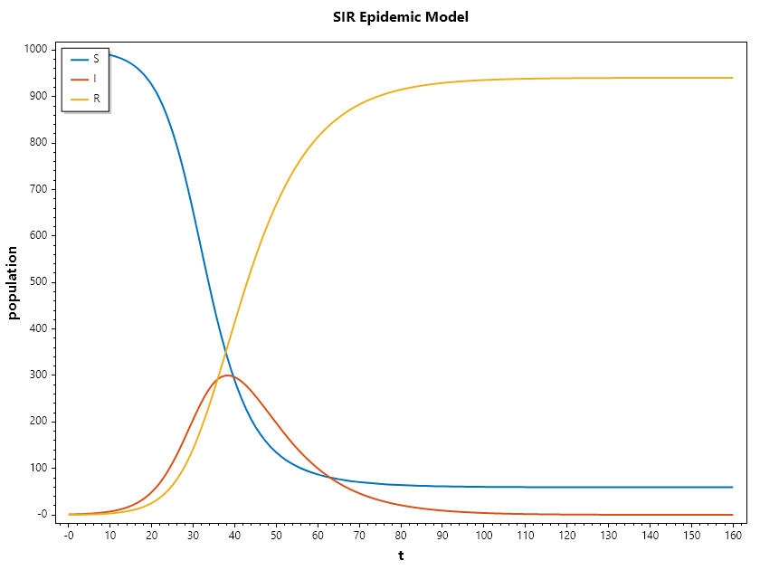
The SIR model divides a population into three compartments: Susceptible (S), Infected (I), and Recovered (R). The model is defined by the following system of ODEs:

\begin{eqnarray} \cfrac{dS}{dt} &= -\beta\cfrac{S I}{N} \\ \cfrac{dI}{dt} &= \beta\cfrac{S I}{N} - \gamma I \\ \cfrac{dR}{dt} &= \gamma I \end{eqnarray}

Example 5C#

// Define the ODE as a function
double betaSIR = 0.3, gammaSIR = 0.1, N = 1000.0;
double[] dydt(double t, double[] y) => [
    -betaSIR * y[0] * y[1] / N,
     betaSIR * y[0] * y[1] / N - gammaSIR * y[1],
     gammaSIR * y[1]];
// Initial condition
double[] y0 = [999.0, 1.0, 0.0];
// Time span
double[] tspan = [0, 160];
// Solve the ODE using Ode45
(ColVec T, Matrix Y) = Ode45(dydt, y0, tspan);
//  Plot the results
Plot(T, Y, Linewidth: 2);
Legend(["S", "I", "R"], UpperLeft);
Title("SIR Epidemic Model");
Xlabel("t");
Ylabel("population");
SaveAs("SIR_Epidemic_Model.png");

OutputFrom the book

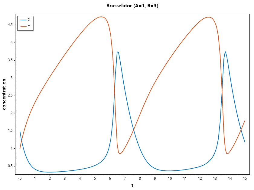
.. Admonition:: Example 5 : Brusselator Model

The brusselator is a theoretical model for a type of autocatalytic reaction. It is defined by the following system of ODEs:

\begin{eqnarray} \cfrac{dx}{dt} &= A - (B + 1)x + x^2y \\ \cfrac{dy}{dt} &= Bx - x^2y \end{eqnarray}

Example 6C#

// Define the ODE as a function
double A = 1.0, B = 3.0;
double[] dydt(double t, double[] y) => [
    A - (B + 1.0) * y[0] + y[0] * y[0] * y[1],
    B * y[0] - y[0] * y[0] * y[1]];
// Initial condition
double[] y0 = [1.5, 1.0];
// Time span
double[] tspan = [0, 15];
// Solve the ODE using Ode45
(ColVec T, Matrix Y) = Ode45(dydt, y0, tspan);
//  Plot the results
Plot(T, Y, Linewidth: 2);
Legend(["X", "Y"], UpperLeft);
Title("Brusselator (A=1, B=3)");
Xlabel("t");
Ylabel("concentration");
SaveAs("Brusselator_Model.png");

OutputFrom the book

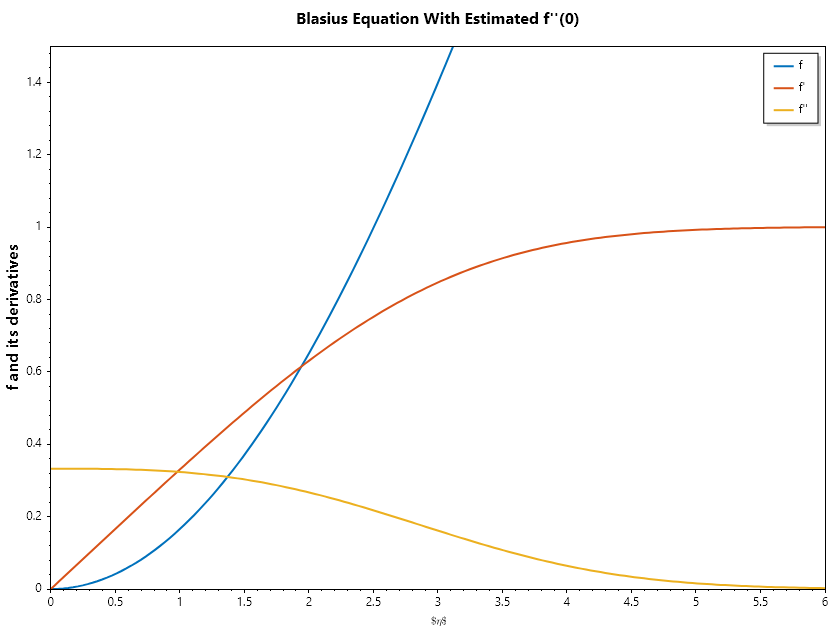
.. Admonition:: Example 6 : Blasius Boundary Layer

The Blasius Boundary Layer refers to a boundary layer of fluid in the vicinity of a flat plate that moves steadily in its own plane.This concept was first introduced by German mathematician Heinrich Blasius. This solution is important in the field of fluid dynamics, particularly in the area of laminar flow.In this solution, the flow velocity outside the boundary layer is assumed to be uniform. Inside the boundary layer, the fluid's velocity changes from zero at the plate surface to the free stream velocity at the edge of the boundary layer. This concept plays a significant role in understanding and predicting the behavior of fluid flow in various engineering and scientific applications. The solutions to the Blasius equation provide valuable insights into the behavior of fluid flow near a boundary. For instance, it demonstrates that the boundary layer thickness grows as the square root of the distance along the plate. Also, it reveals that the shear stress at the plate surface is proportional to the square root of the free stream velocity, among other observations. The Blasius Boundary Layer solution, despite its simplifications, offers a good approximation for real-life engineering problems involving fluid flow over flat surfaces.This understanding is crucial in designing and optimizing various engineering systems, ranging from airfoils in aeronautics to heat exchangers in thermal power plants and thermal shield design on reusable rockets.

2f''' + f''f = 0

This equation can be solved by transforming it into a system of 1st order differential equations. Let: $y_1 = f, y_2 = f', y_3 = f''$ hence

\begin{array}{rcl} y'_1&=&f' = y_2, \\ y'_2&=&f'' = y_3, \\ y'_3&=&f''' = -0.5f''f = -0.5y_3y_1 \end{array}

So, the system of first order differential equation is thus:

\begin{array}{rcl} y'_1&=& y_2, \\ y'_2&=& y_3, \\ y'_3&=& -0.5y_3y_1 \end{array}

Subject to the following initial and terminal conditions. $y_1(0) = 0, y_2(0) = 0, y_2(\infty) = 1$ To solve system of ordinary differential equation, you need the initial conditions, but when one of the initial conditions is missing, and we have a terminal condition instead, we can solve for the initial condition we do not have using the terminal condition we have, just like finding the root of a nonlinear function.But to evaluate the value of the function that you want to be zero, you have to perform the integration of the ode, using the guess given by the nonlinear solver and then return the function value which is the difference between the terminal value you obtained from the integration and the desired value.In this case the unknown value is $y_3(0)$ , and the function value is $y_2(\infty) - 1$ .

Example 7C#

ColVec T = null; Matrix Y = null;
double err(double alp)
{
    (T, Y) = Ode45((t, y) => [y[1], y[2], -0.5*y[0]*y[2]], [0, 0, alp], [0, 6]);
    return Y[^1, 1] - 1;
}
//Use a root finding method to find the value of alp that satisfies the boundary condition at t = 6
double alp = Fsolve(err, 0.5);
//Compare with the solution of the BVP using a direct method
Console.WriteLine($"Solution is {alp}");
//Plot the solution
Plot(T, Y, Linewidth: 2);
Legend(["f", "f'", "f''"]);
Axis([0, 6, 0, 1.5]); 
Xlabel("$\\eta$", interpreter: Latex ); Ylabel("f and its derivatives");
Title("Blasius Equation With Estimated f''(0)");
SaveAs("Blasius-bounary-layer.png");

OutputFrom the book

Solution is 0.33256562390833655