Solution of Linear Systems

Solving a system of linear equations is the most fundamental task in computational science. The goal is to find the vector :math:x that satisfies the relationship between the coefficient matrix :math:A and the result vector :math:b.

1. Direct Methods

Direct methods aim to find the exact solution (within rounding error) in a finite number of steps.

• Gaussian Elimination: The classic method of transforming :math:A

into an upper triangular matrix using row operations. LU Decomposition: As discussed previously, factorizing :math:A = LU is the standard approach for systems where :math:b changes but :math:A remains constant. Cholesky Decomposition: A specialized, faster version of LU for matrices that are symmetric and positive-definite.

// Solve linear system of equations
Matrix A = new double[,] 
{ 
    {  1,  1,  1,  1 },
    {  2, -1,  3, -1 },
    { -1,  4, -1,  2 },
    {  3,  2,  2, -1 }
};
ColVec b = new double[] { 10, 5, 8, 20 };
ColVec x = Mldivide(A, b);
Console.WriteLine($"A = \n{A}");
Console.WriteLine($"b = \n{b}");
Console.WriteLine($"x = \n{x}");

A = 

 1   1   1   1 
 2  -1   3  -1 
-1   4  -1   2 
 3   2   2  -1 

b = 

10 
 5 
 8 
20 

x = 

   6.9130
   2.2174
  -1.4348
   2.3043

. 2. Iterative Method

SepalSolver provides two major iterative solvers. Conjugate Gradient (ConjGrad) for large sparse symmetric matrices and the Generalized Minimum Residual (GenMinRes) for large sparse nonsymmetric matrices.

.. Admonition:: Example 1 : Generalized Minimum Residual

This eaxample shows how to use generalized minimum residutal method. Pay attention to how the Matrix was made.

int n = 1000;
ColVec a = Ones(n-1), b = Ones(n), e = -a, c = 2 * e;
ColVec d = -10 + 3 * b;
Matrix A = Diag([e, d, c], [-1, 0, 1]);
var (x_iter, flag, res, iter, resvec) = GenMinRes(A, b, 1e-6, 20);
Console.WriteLine($"x = {x_iter[..10].T}...{x_iter[^10..].T}");
Console.WriteLine($"flag = {flag}");
Console.WriteLine($"iter = {iter}");
Console.WriteLine($"res = {res}");

x = 
  -0.1149   -0.0978   -0.1003   -0.1000   -0.1000   -0.1000   -0.1000   -0.1000   -0.1000   -0.1000
...
  -0.1000   -0.1000   -0.1000   -0.1000   -0.0999   -0.1002   -0.0992   -0.1027   -0.0911   -0.1298

flag = 0
iter = 9
res = 3.6283012552149887E-07

.. Admonition:: Example 2 : Conjugate Gradient

This eaxample shows how to use conjugate gradient.

int n = 1000;
ColVec a = Ones(n-1), b = Ones(n);
ColVec d = -5 +  b;
Matrix A = Diag([a, d, a], [-1, 0, 1]);
var (x_iter, flag, res, iter, resvec) = ConjGrad(A, b, 1e-6, 20);
Console.WriteLine($"x = {x_iter[..10].T}...{x_iter[^10..].T}");
Console.WriteLine($"flag = {flag}");
Console.WriteLine($"iter = {iter}");
Console.WriteLine($"res = {res}");

x = 
  -0.3660   -0.4641   -0.4904   -0.4974   -0.4994   -0.5000   -0.5000   -0.5000   -0.5000   -0.5000
...
  -0.5000   -0.5000   -0.5000   -0.5000   -0.5000   -0.4994   -0.4974   -0.4904   -0.4641   -0.3660

flag = 0
iter = 6
res = 8.189558921548075E-07

. 3. Overdetermined Systems (Least Squares)

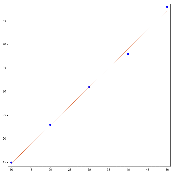
SepalSolver also perform compute least square solution when the number of rows exceed number of columns. .i.e, where there are more equations than variables being solved. Sepalsolver would compute a least square solution to the problem by transforming Ax = b into A^TAx = A^Tb, which now has equal number of equations and variable. When there are more equations than unknowns (common in data fitting), there is often no "perfect" solution. We instead find the x that minimizes the error ||Ax - b||^2.

Consider a phenomenon in which temperature and pressure are linearly related. i.e P = mT + e. Even though there are just 2 variables, we have 5 measurements.

Example 4C#

Copy Code

1

2

3

4

5

6

7

8

9

10

11

12

13

14

15

16

// Data
double[] T = [10, 20, 30, 40, 50];
double[] P = [15, 23, 31, 38, 48];
​
// Construct least square problem
Matrix A = T.Select(t => new RowVec([t, 1])).ToList();
ColVec b = P;
​
// Compute m and e
var x = Mldivide(A, b);
Console.WriteLine($"m = {x[0]}, e = {x[1]}");
​
Scatter(T, P, "fob"); HoldOn();
Plot(T, A*x); HoldOff();
​
SaveAs("LeastSquare-Solution.png");

// Data double[] T = [10, 20, 30, 40, 50]; double[] P = [15, 23, 31, 38, 48]; // Construct least square problem Matrix A = T.Select(t => new RowVec([t, 1])).ToList(); ColVec b = P; // Compute m and e var x = Mldivide(A, b); Console.WriteLine($"m = {x[0]}, e = {x[1]}"); Scatter(T, P, "fob"); HoldOn(); Plot(T, A*x); HoldOff(); SaveAs("LeastSquare-Solution.png");

OutputFrom the book

m = 0.8099999999999999, e = 6.700000000000002

3. Matrix Condition Number

A system is "ill-conditioned" if a tiny change in :math:b causes a massive change in :math:x. This is measured by the Condition Number :math:\kappa(A).

• Low \kappa: Stable system.
• High \kappa: Unstable; numerical solutions may be garbage.